Internal Assessment for IB Physics HL
Topic: How does distance from a wire affect the field strength produced by the wire?
Testing session: May 2023
Word count: 2271
Table o’ contents
Main stuff:
Introduction (c’mon man you know what an intro is)
Method (how I did what I did)
Results (what I got from what I did)
Evaluation (why I did what I did)
Bibliography (Who helped me did what I did (Murray isn’t on there but he also helped a lot))
Additional Stuff:
Set up/diagram (super cool)
Equation (also super cool J)
Speed data (wheeeeee)
Average Field Strength Vs. Distance Graph (og graph)
Log v Log graph (the epic battle)
Linearized graph (oh mama)
Excel Data for all graphs Text Version (hope it helps)
Related sites (also hope it helps)
Some of the units that IB students find themselves working through on the road to becoming a physicist are the electronics and magnets units, both of which admittedly tested my mathematical skill and conceptual thinking ability to quite the extent, and quickly became some of my favorites. Although I enjoyed a great deal of the units we have gone through throughout physics; such as kinematics, fluid dynamics, and thermodynamics, since I have been young I have had a particular interest in both magnetism and electricity. As a child my parents had to intervene incredibly frequently as my two toys of choice were a set of magnets my brother had gifted me from a local science institute and a build-your-own circuit and electricity set my grandparents had gotten me for the holidays, two famously dangerous toys for a child under ten, but so be it. The magnets served as something of a curious hobby, whereas the circuits became more of a focus as I was fairly certain that I wanted to be an electrical engineer at some point in my later life. This was until I discovered that the blending of these two hobbies; electronics and magnets, had some pretty detrimental results usually in the realm of the magnets destroying whatever electronics I was hoping to work with; a notion that would be re-iterated upon my taking a job in tech support where we manually erased hard drives with magnets.
This intrigue only grew in my IB physics class, when we learned about Oersted’s law which states that a current carrying a wire makes magnetic fields.
So this notion that electricity itself, in the form of currents, can create its own magnetic field became of great interest to me, if we use these components such as wires that carry currents throughout them, which in turn produce their own magnetic fields, how is this not ultimately damaging to the devices they are within? What determines the strength of these magnetic fields?
Now my hypothesis is that as you move further from the magnetic field, the field strength will decrease, as is common with non electro-magnetic fields, however I am still curious as to how much and how fast it will decrease, as the computers that these components go into are incredibly tightly packed and if the relationship is linear, which I believe it will be, means there is an incredibly small margin of error in designing laptops. In order to determine this relationship I will be using an independent variable of the distance the magnetic field is from what is measuring it, and increasing it over time to test the field strength, meaning the field strength will serve as my dependent variable.
Materials used: 50 ft of wire, duct tape, meter stick (with cm and mm markings), computer, Vernier logger pro, transformer, cables, Hall effect probe
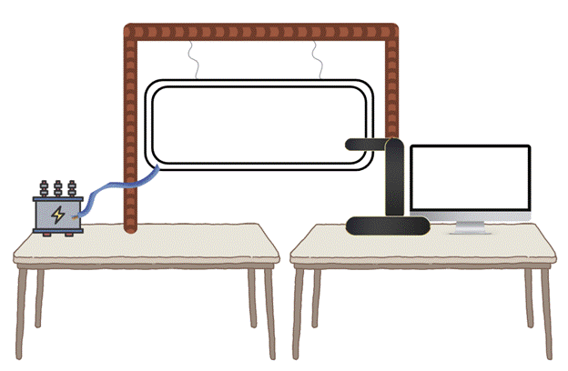
Procedure: For this experiment I connected a large loop of wire that was suspended in air by hanging, to a transformer that allowed me to manually adjust the current, which was set at 5 amps. Then using a computer with the Vernier LoggerPro program running on it, I set up the Hall effect probe which would give me a reading of the magnetic field strength it was experiencing, in this case the field it would be reading the field given off by the current traveling through the wire. I set this program to record 20 readings a second for an interval of 5 seconds, in order to measure the field strength at varying distances. For the remainder of the experiment I would align the Hall effect probe along the meter stick which I had taped to the desk to ensure it would not move, for each trial I would move it half a centimeter further from the wire, thus serving as how I manipulated my independent variable. I would then press start on the computer program and allow it to record data for the allotted 100 data points (20 data points a second for 5 seconds), from which I would record the maximum, minimum, and mean field strength at that distance interval. I chose this many data points as in experimental electro-magnetic physics it is more than likely that the exact current would fluctuate slightly, especially given that the technology I was working with is on the older side, and the more data points I could capture and average, the more likely my data was to be accurate. After each trial I would check to make sure the transformer was still set firmly at 5 amps in order to ensure my control variable stayed constant throughout the entirety of the experiment. I utilized my .5 cm increments from 1 cm to 15 cm, both for time constraint and manageable data constraint purposes, as this gave me 29 data points once averaged. As for the safety concerns of my experiment, both the low amperage and insulated nature of the wire allowed me to fairly successfully avoid any shocking instances, although admittedly several of my peers, fascinated in what I was doing, asked “hey is that hot?” before placing their hands on the wire, to which the answer was, yes, yes it is hot. Luckily word-of-mouth travels fast in a physics laboratory and after only one or two incidents all had learned from other’s mistakes.
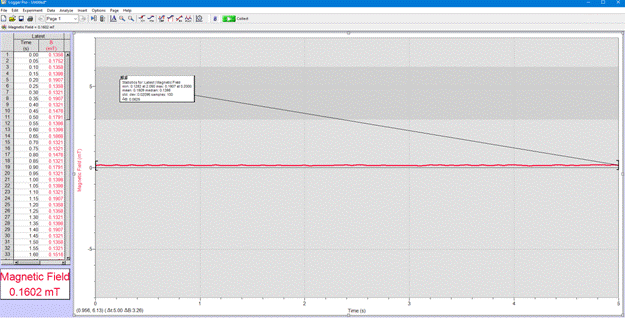
Here is a screenshot from the data acquisition phase. Using the Vernier logger pro program I was able to automatically record the field strength 20 times a second for 5 seconds, the computer would then produce an average of all 100 of those data points, as well as the highest (maximum) and lowest (minimum) readings during the 5 second period. I repeated this process for each of the distance increments, and that is what brings us to the data table below!
Above is the processed data from the data acquisition phase. The average field strength was automatically calculated by the program from the 100 data points it gathered during the 5 second measuring phase. The uncertainty was calculated by hand by taking the minimum measurement and subtracting it from the maximum measurement, then dividing that value by 2 in order to determine the uncertainty. For instance, the uncertainty calculated from the 10 cm data point was the maximum value, 0.3514, minus the minimum value, 0.2695, giving us 0.3514 - 0.2695 = .0819. Then dividing this value by 2 in order to give us .0819 / 2 = 0.04095 which is the uncertainty.
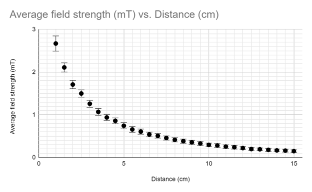
Here is a graph of the processed data complete with error bars representing the uncertainty of each data point. Based on the curvature of this graph my initial assumption was that we were looking at an exponential decay, which does go against my hypothesis that the relationship between distance and strength would be linear.
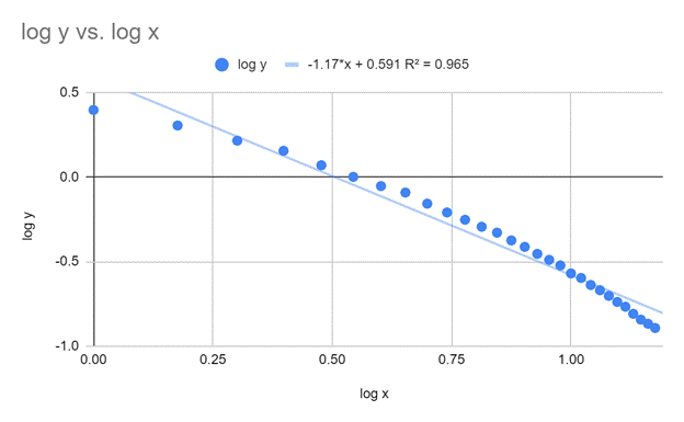
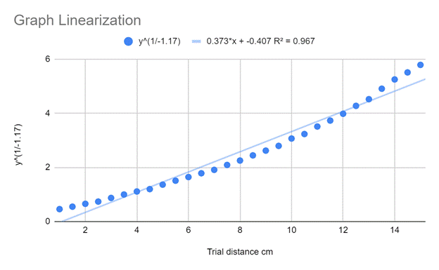
Since it appeared I was working with some form of power function, in order to obtain a better understanding of how the relationship was modeled I decided to linearize the graph. My attempt to linearize the graph consisted of taking the log value of both my y value and my x value, which theoretically would have provided me with a linearized graph with an equation in y = mx + b format in which the m value would be the exponent in the original power function seen in Graph A. After completing this step I was left with the graph you see above, which provided me with an original exponent of -1.17. Somewhat confused as to what this would mean, it was at this point in the investigation I began to turn my attention to Ampere’s law. Ampere’s law, discovered by André-Marie Ampère in the early nineteenth century, is the law that states that “the magnetic field created by an electric current is proportional to the size of that electric current with a constant of proportionality equal to the permeability of free space” (byjus.com), and is most commonly used as a way of determining either the electrical current being carried through a wire via the magnetic field or produces, or vice versa measuring the magnetic field produced by a wire via measuring the current being carried throughout said wire. Essentially; Ampere’s law gives us a way to translate between electrical and magnetic aspects of physics mathematically, and is modeled as;
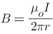
and can supposedly calculate the strength of the magnetic field about the wire if you have the dimensions of the wire, as well as the current flowing through it. Which is why upon further examination of Ampere’s law, this inverse relationship actually began to make quite a bit of sense, as the law is modeled by the equation, B = (μ0 I)/(2πr), which while at first admittedly seems rather complicated, almost every variable in that equation either is a constant or can be kept constant. μ0 is the permeability constant, both 2 and π are constants, and in using the current as a control variable we effectively made I a constant as well, meaning the only variable that was not a constant is r, meaning if you remove all of the constants from the equation the variable in which you are altering the equation by effectively becomes 1/r. Which could also be written as r^-1, which is the exponent I discovered via this linearization. The only issue with this discovery lies in the fact that the graph above is not linear. Although the graph has a satisfactory r value of 0.965, upon visual inspection it is clear that it does not follow a linear trajectory, as a properly calculated linearized graph should. After double (and possibly quadruple) checking my calculations, I was certain that had not been the source of error. To obtain a more holistic picture I decided to make a graph in which my original y value was raised to this new exponent, which is the graph you see below.
From here I became thoroughly confused, as again this data was not appearing visually linear, despite having a reasonable r value. Although here the m value of 0.373 caught my eye as it appeared abnormal. After revisiting my setup, and extensive research into how the program I was using operated, I have determined it is likely that there was a 0 error upon the initial setup of my experiment that offset the data by approximately 0.3. In order to remedy this error, I created a graph of my data in which I raised it by 0.3 which produced the graph you see below.
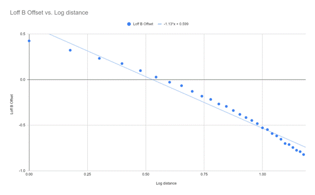
This graph does appear more linear, while maintaining the original exponent of around -1 that was hypothesized earlier to be the relationship between the magnetic field and the distance from the wire when considering the constants within Ampere’s law.
Which means I am rejecting my original hypothesis that the relationship between the magnetic field and the distance from it is a linear relationship, and instead positing that because all other variables within Ampere’s law are constants, the relationship between the magnetic field strength and the distance from the wire is proportional to r^-1, which does adhere to Ampere’s law.
Holistically this experiment allowed myself for much greater insight into the inner workings of Ampere’s law, although that is not to say it is without issue. Perhaps my greatest error was the 0 error that entirely altered my data and subsequently the curvature and linearize-ability of my graphs. In all honesty, I am not entirely sure how one would remedy this 0 error as I did attempt to 0 the program (as instructed by the program guidelines) before beginning my experiment, it is possible it is a product of well-loved and older equipment, or perhaps there is simply a limit on the ability to 0 the data as the measuring device can only be so close to the current as the wire was insulated for safety purposes.
In order to determine if my new-found hypothesis that the relationship between magnetic field strength and distance is proportional to r^-1 bares any replicability it would be interesting to repeat this experiment with a variety of different currents, as well as perhaps the effect an unstable current would have on a magnetic field as well.
The notion that the relationship is proportional to r^-1 would make sense in regards to computer design when it comes to protecting internal components that may be easily damaged by magnetic fields as it means miniscule alterations in distance can have large effects on the field strength.
“André-Marie Ampère.” Encyclopædia Britannica, Encyclopædia Britannica, Inc., 16 Jan. 2023, https://www.britannica.com/biography/Andre-Marie-Ampere.
Admin. “Ampere's Law - Definition, Statement, Examples, Equation, Video, Applications and Faqs.” BYJUS, BYJU'S, 3 Feb. 2023, https://byjus.com/physics/amperes-law/#:~:text=Ampere's%20law%20states%20that%20%E2%80%9CThe,the%20permeability%20of%20free%20space.%E2%80%9D.
A good overview of Ampere’s law: http://hyperphysics.phy-astr.gsu.edu/hbase/magnetic/amplaw.html
Way more info then you could ever need on Ampere’s law: https://en.wikipedia.org/wiki/Amp%C3%A8re%27s_circuital_law
Where I got my definitions and basis: https://byjus.com/physics/amperes-law/
A good place for laws closely related to Ampere’s law: https://www.britannica.com/science/Amperes-law
Pretty neat slideshow about it (Illinois you’ve done it again): https://web.iit.edu/sites/web/files/departments/academic-affairs/academic-resource-center/pdfs/Amperes_law.pdf
Thanks for reading my site! I hope you enjoyed and if you’re an IB Physics student struggling with your IA, stay strong, it’ll turn out better than you thought and you might even enjoy it! <3