The Differential Rate of Change of Water Depth in a Leaking Bucket
Maxwell Siebersma
Table of
Contents
1. Introduction
2. Methods
3. Results
4. Analysis
5. Conclusion
Introduction .:. Top
Differential equation modeling is an invaluable tool in physics to understand
how relations between variables change, especially with respect to time. It is
rather elementary to determine instantaneous forces and velocities, but more
difficult to determine how these factors change with time. Differential
equations provide the means to analyze how these factors are related, and
ultimately can give a model for a system. In this experiment, I analyzed the
change in the height of water in a leaking bucket with differential equations.
This has wide reaching applications in engineering, as many mechanical systems
depend on consistent fluid flow in order to operate. It may initially seem
simple to determine this rate of change. Most simply, the change in height over
time can be given with the equation ![]() , where A1 is the area
of the bucket, A2 is the area of the hole, and u is the velocity of
the water exiting the bucket. The velocity is highly variant over time due to
pressure- when the water is at full height, the pressure is highest, but the
pressure gradually decreases as water flows out of the bucket and the depth
decreases. Using pressure equations in fluid dynamics and assuming an even
cylindrical bucket, I solved the differential equation of height with respect
to time below:
, where A1 is the area
of the bucket, A2 is the area of the hole, and u is the velocity of
the water exiting the bucket. The velocity is highly variant over time due to
pressure- when the water is at full height, the pressure is highest, but the
pressure gradually decreases as water flows out of the bucket and the depth
decreases. Using pressure equations in fluid dynamics and assuming an even
cylindrical bucket, I solved the differential equation of height with respect
to time below:
![]() →
→ ![]()
![]()
![]()
![]()
![]()
Given that the water had an initial height of 0.4m, the bucket’s radius was 0.15m, the hole’s radius was 0.01m, and gravitational acceleration in 9.81 ms-2, the equation can be simplified to the following equation, where t is in seconds and h is in meters.
![]()
This model indicates a mostly linear initial decrease in height until the t2 component is large enough to take effect and slow the rate of change until both the height and the derivative simultaneously reach 0. A graph of this equation can be seen below.
The primary aim of this experiment was to determine the accuracy of this differential model by testing with an actual bucket of water with a hole. I hypothesized that this model would true, with a polynomial regression of the results being similar to the equation.
Methods .:. Top
Materials
-Cylindrical Bucket (40 cm or greater in height, 15 cm radius), with small hole cut into bottom (1 cm radius)
-Water
-Rubber Stopper (1 cm radius)
-Knife
-Meter Stick
-Super Glue
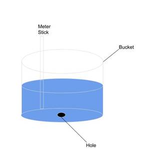
To conduct this experiment, a plastic cylindrical bucket with a height slightly greater than 40 cm was used (the bucket’s total height is obsolete so long as it was at least 40 cm). An outlined circle of radius 1 cm was cut out of the bottom using a knife. A meter stick was attached to the inside of the bucket using super glue; this was determined to have negligible effects on the displacement of the water. A rubber stopper was firmly placed in the hole to prevent water from leaking before the experiment. The water was poured into the bucket to a height of 40 cm. Once the rubber stopper was removed, a timer was started. At 5 second increments, I recorded the height of the water using the meter stick. A diagram of the experimental setup can be seen below.

The dependent variable for this experiment was the height of the water in the bucket. This was an indiscrete value, but was measured at discrete time intervals in centimeters. The independent variable for the experiment was time. Rather than being a manipulated variable, the height was measured with respect to the natural flow of time in order to test the model h(t). Controlled variables include many of the constant terms from the differential equation- the same bucket with the same radius and hole were used, water was used in each trial, and the initial height of the water was constant.
Results .:. Top
The following is a graph of the results between the three trials. Although the original equation used height in meters, centimeters were used instead because the heights were originally measured in centimeters, and it provides a higher ease of graphing and calculations. Fitting with the original model, a 2nd degree polynomial was used for the regression line. On the graph, the equations for the individual trials are given. Between all trials, the regression equations were highly similar. Additionally, the error bars for the results are given on the graph. The error bars are highest in the towards the earlier times, but continue to decrease as time progresses and height decreases.
R2 = 0.991
The R2 value is exceptionally high for the results, indicating a strong trend towards the regression polynomial. A table of uncertainties for the results are included in the table below. The results between the three trials were very similar at each time increment; as such, the uncertainties were in large part quite low.
Uncertainty of Results Between Trials
|
Time (s) |
Uncertainty |
|
0 |
0 |
|
5 |
士0.45 |
|
10 |
士0.35 |
|
15 |
士0.25 |
|
20 |
士0.25 |
|
25 |
士0.15 |
|
30 |
士0.15 |
|
35 |
士0.15 |
|
40 |
士0.25 |
|
45 |
士0.20 |
|
50 |
士0.15 |
|
55 |
士0.20 |
|
60 |
士0.15 |
|
65 |
士0.05 |
|
70 |
0 |
In order to mathematically test the validity of the original differential equation, the coefficients of the quadratic equation can be compared for similarity. The coefficients are named A, B, and C, corresponding to those in the polynomial f(t) = At2 + Bt + C. In the following table, the coefficients from the theoretical model is compared to the coefficients computed from the data.
Coefficients of Original Model vs. Regression Results
|
|
Theoretical Model |
Trial 1 |
Trial 2 |
Trial 3 |
Average |
|
Coefficient A |
0.009689 |
0.00962 |
0.00994 |
0.00959 |
0.00972 |
|
Coefficient B |
1.245 |
1.25 |
1.27 |
1.25 |
1.26 |
|
Coefficient C |
40.00 |
40.2 |
40.7 |
40.4 |
40.5 |
To compare the coefficients to the theoretical model accurately, the percent errors of the trials and the average of the results are provided in the table below.
Percent Errors of Equation Coefficients Between Trials
|
|
Trial 1 |
Trial 2 |
Trial 3 |
Average |
|
Coefficient A |
0.71% |
2.59% |
1.02% |
0.31% |
|
Coefficient B |
0.40% |
2.01% |
0.40% |
1.20% |
|
Coefficient C |
0.50% |
1.75% |
0.50% |
0.63% |
In the individual trials, coefficient A seemed to have higher percent errors. However, with the average of all the results, coefficient B had the highest percent error. Additionally, Trial 2 seemed to have higher percent errors overall than trial 1 or trial 2. In all, the percent errors were fairly low. This indicates that the theoretical model from the differential equation is highly accurate in predicting the actual results of the data.
Conclusion .:. Top
Overall, the results of the experiment supported my hypothesis that the height would reduce at a rate given by the equation h(t)=0.00009689t2 - 0.01245t + 0.4. The percent error between the coefficients of the regression and the coefficients of the theoretical model were low, indicating that the model fit the data exceptionally well. There was significant correlation between the values predicted by the differential equation and the actual values. The differential equation was conclusively successful in modelling the decrease in the height of the water.
There were some sources of error throughout the experiment. Perhaps the most significant was the rudimentary method of data collection- it was done with a timer, by sight, using a meter stick. With the limitations of human ability, it is to be expected for there to be some error in data collection itself. The deviation in trial 2 was likely due to this error, as my timing and recording was more inconsistent during this trial than the other two trials. However, there was also some pattern to the errors in the data. In the automatically calculated error bars in the graph and in the uncertainties, the data was less precise in earlier time frames than later time frames. Additionally, coefficient B had the highest average percent error of the coefficients. In part, this could be attributed to the fact that the values of height were higher, suggesting greater variability. Underlying this, though, is the possibility that the flow for these early values was more chaotic. Reynold’s numbers, a measurement of the turbulence of a fluid flow, are proportional to the fluid’s flow velocity. Initially, the pressure of the water was higher, leading to a higher velocity of the water expelled from the bottom. The equations for fluid flow are only accurate for laminar flows. Because the flow was faster and more turbulent initially, there was greater inconsistency in the velocity. Nevertheless, the values were still quite accurate, and the flow was likely laminar to a greater extent.
In the end, I was surprised by how accurately my differential equation was able to map the change in the real world. Although the creation of the setup was rudimentary, the mathematics lined up with the physical world in a stunning way. Future experimentation could explore how this relation changes with different fluids. I was surprised by how density was cancelled in the equation and viscosity did not appear, and it surprised me that my results were accurate without these variables. I am curious as to whether the accuracy would be marred by a fluid of greater viscosity or density.
It was amazing to see
physical results line up with theories and mathematics. In this experiment, I
was able to see firsthand how mathematics can be a powerful tool to explain the
phenomena we see in nature.
Annotated
Sources
.:. Top
https://sciencing.com/calculate-flow-through-hole-pipe-5885513.html- This source contains useful information on the flow rate of water through a pipe or hole assuming a constant pressure, which is useful to know before tackling changing pressure
https://www.math.hmc.edu/calculus/tutorials/odes/- This source is useful for learning the use of first order differential equations, which are used above in this paper
https://www.britannica.com/science/Torricellis-theorem- This site provides information on Torricelli’s principle, which gives the velocity of a fluid at v=sqrt(zgh), derived above from Bernoulli’s theorem
https://www.youtube.com/watch?v=eNqDwrprcKE- This video uses differential equations in the same manner used in the above equations with Toricelli’s principle to find the polynomial flow rate from a bucket with a hole
https://www.youtube.com/watch?v=KhsbeI9QPls- This video similarly uses differential equations to find the function of height related to time as water drains from a tank (using a cylindrical tank similar as to that in this paper).
https://www.youtube.com/watch?v=8n5bIZkLov8- This source was useful in the methodology of the experiment, specifically in assisting in the cutting a hole in the bottom of the bucket that was almost circular.