INTRODUCTION:

Katie and Mary's Battle With

Simulacra!!!!

Elephant / Lightning

Table of Contents

Discussion/Conclusion

Bibliography

Related Links

Return to Research Page

INTRODUCTION:

Cellular automata are “computer simulations that try to emulate the way the laws of nature are supposed to work in nature” (Ehrencrona). Cellular automata may not necessarily be completely accurate all of the time, but they do provide some answers as to how an organism reacts towards its environment. Cellular automata also may illustrate the ways certain diseases behave such as Cancer. Furthermore, the cellular automata is a community of cells which interact with one another. Thus, the cellular automata serves to depict both population and community ecology since it incorporates the interactions of different cells within a pattern. The cells behave in a way that depending on the location of one cell, a neighboring cell will either survive, become deactivated and “die,” or be born.

There are several essential features of cellular automaton. These include: its state, which can either be a number or a property; its neighborhood, which consists of the cells with which it interacts; and its program, which defines the changes that it endures in response to its status and that of its neighbors. The state, explained in biological terms, could represent “the number of animals at each location or the type of forest cover growing there…if each cell represents part of a landscape” (Green). Furthermore, the states could correspond to environmental features such as coral cover or topography. Cellular automata also possess several properties, which consist of self-organization, life-like behavior, and “thermal” behavior. In self-organization, patterns are forced to emerge. Furthermore, in life-like behavior, the automata behave in ways like those of biological systems. For example, the cells may: “die out, become stable or cycle with a fixed period, grow indefinitely at a fixed speed, or grow and contract irregularly” (Green). In thermal behavior, configurations may either be frozen into a stable pattern or may behave in a more active, gaseous way.

In cellular automata, several items can be altered. These include: the number of states per cell, the number of dimensions, the way cells are arranged, the neighborhood, the weight of neighbors, and the operations performed on neighbors (Wójtowicz). In addition, the parameters can be altered, the birth and survival rates changed, by selecting a different number that a cell requires to be born or to survive. Although the typical birth/survival numbers are 3, and 2 and 3, these numbers can be altered so that the birth/survival numbers could be 5, and 4 and 7.

The game of LIFE was invented by the mathematician John Conway. In this program, a cell is either alive or dead, and the effect of a cell’s neighbors’ location is determined as it is this that determines whether or not the cell is alive or dead. This is supposed to be reminiscent of population change. In this program the rules are:

1. A living cell with only 0 or 1 living neighbors dies from isolation.

2. A living cell with 4 or more living neighbors dies from overcrowding.

3. A dead cell with exactly 3 living neighbors becomes alive.

4. All other cells remain unchanged.

However, as mentioned above, these numbers may be altered. The standard is what we listed in 1-4, but by altering the parameters, we can adjust the birth/survival numbers to any number we want to. (The survival rate represents the number of neighbors a cell needs to survive, and the birth rate represents the number of neighbors for a cell to come to life.) As the generations pass, cells either are maintained in some type of order, broken up into isolated patterns, or disappear.

In the Life program, the number of states can be altered in addition to the survival and birth rates. Within my experiment, the state refers to the state of the cell. A cell with two states would be considered either “alive” or “dead.” A cell with 8 states would be either “dead” or seven shades of alive. In the case of our cellular automata viewer (CAV), the states are represented by different colors or different shades of color. To illustrate this, imagine the states representing the forest cover (and its different stages), and after examining the effects of a forest fire, the states could represent the different stages a forest progresses through including bare earth, grass, woodland, and closed forest.

Preston and Duff write, “ Conway. . . discovered a simple rule which had an immediate effect, i.e. led eventually to either a stable pattern or to patterns exhibiting a repetitive, i.e. oscillatory, stability” (10). Although it is evident that the different programs within the cellular automata viewer do emerge as patterns, whether stable or completely random, we would like to pursue the effects of altering a parameter, the number of states. We would like to see what effect this would have on the original pattern. Thus, we intend to manipulate the states to see if a cycle emerges in the population.

Statement of the Problem:

What will happen when the states of a pattern are altered in an environment where the birth and survival rates equal zero?

Statement of the Hypothesis: If we increase the number of states in a pattern, then it will cause an increase in the number of generations within a cycle.

METHOD:

We began by downloading the cellular automata viewer 2.0 CavGB from the site: http://www.rennard.org/alife/english/cavgb.html. Since we were fairly inexperienced with this program, we learned the basics of how to use it by using the help section and figuring out what all of the different devices in the main bar and the control panel represented. Out of the four available programs for cellular automata (Life, Vote, 1D Wolfram, and 1DB Langton), the Life mode seemed the most appealing. Next, we figured out how to alter the birth, survival, and state rates. We also learned how to change the dimensions (the size of the cells), the speed, whether or not it ran all at once or step by step, and how to save a pattern which we created.

We created my pattern by selecting a “random” scattering of data under dimension one (which zooms in on the cells). Once we had created our own pattern, and saved it as “JINX,” we then altered the birth, survival and state rates. We chose to select zero for both the birth and survival rates. Since we had set out to determine the effects of the states on the population, we kept the survival and birth rates at zero throughout the entire lab, but we changed the states. The states thus served as the independent variable which would alter the dependent variable, the population.

In the JINX pattern, we first found the population numbers for the first thirty generations after we altered the state number. Once the birth and survival rates were at zero, we began tracking data on Excel for the second state. Then we changed to the third state and tracked the next set of data. We continued to do this for each state. As soon as we had collected all of the data concerning each generation’s population under the seven different states, we then observed at what point the numbers in the population became a cyclic pattern. We then further analyzed what happened when the population did emerge as a repetitious cycle.

Since we wanted to have multiple trials, we decided to run three other trials, one of which we created. We ran the patterns: Oscillator 01, Acorn, and our creation, panda. We did the same thing with these three patterns as we did with JINX. However, with some of these patterns, we had to track the population numbers past the thirtieth generation because it took longer for a population to emerge as a cyclic pattern. Once the patterns did have repetitious cycles, we marked what these cycles were and what population numbers were contained within these cycles. Since the third state never proved to have a repetitious cycle, we continued to run it until the 600^th generation. When we had all of my data compiled on to Excel, we then produced graphs to analyze and compare the data.

Overall, we observed the effect the alteration of the states had on the population. We wanted to see what would happen when we increased the states and whether or not it would take longer for the population to become cyclic.

RESULTS:

Below is the data representing the population numbers at each generation for each different state. The numbers in bold signify where the repetitious cycle begins. The highlighted portions indicate the repetitious cycle.

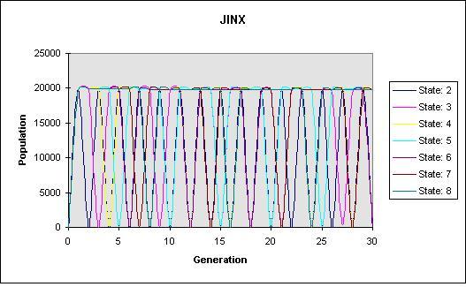
JINX

data file

(started out with an even population)

Generation	State: 2	State: 3	State: 4	State: 5	State: 6	State: 7	State: 8
0	34	34	34	34	34	34	34
1	19831	19855	19855	19855	19855	19855	19855
2	52	19849	19873	19873	19873	19873	19873
3	19831	54	19874	19898	19898	19898	19898
4	52	19819	67	19880	19904	19904	19904
5	19831	19804	19870	79	19886	19913	19913
6	52	84	19857	19867	74	19889	19913
7	19831	19796	19872	19853	19843	74	19889
8	52	19763	66	19874	19824	19867	74
9	19831	102	19870	19858	19829	19848	19867
10	52	19749	19856	69	19824	19853	19848
11	19831	19738	19869	19863	19826	19848	19853
12	52	143	66	19848	44	19850	19848
13	19831	19703	19861	19869	19818	19848	19850
14	52	19711	19853	19858	19816	43	19850
15	19831	174	19867	69	19822	19842	19848
16	52	19658	66	19863	19820	19840	43
17	19831	19676	19863	19848	19822	19846	19842
18	52	210	19851	19869	44	19844	19840
19	19831	19606	19867	19858	19818	19846	19846
20	52	19637	66	69	19816	19844	19844
21	19831	242	19863	19863	19822	43	19846
22	52	19557	19853	19848	19820	19842	19846
23	19831	19606	19865	19869	19822	19840	19844
24	52	296	68	19858	44	19846	43
25	19831	19486	19859	69	19818	19844	19842
26	52	19539	19851	19863	19816	19846	19840
27	19831	367	19865	19848	19822	19844	19846
28	52	19425	70	19869	19820	43	19844
29	19831	19489	19863	19858	19822	19842	19846
30	52	435	19849	69	44	19840	19846

Here is a graph of JINX representing the data from the table above. Its periodic nature shows its cyclic nature. This periodic nature displays the life-like behavior of cellular automata.

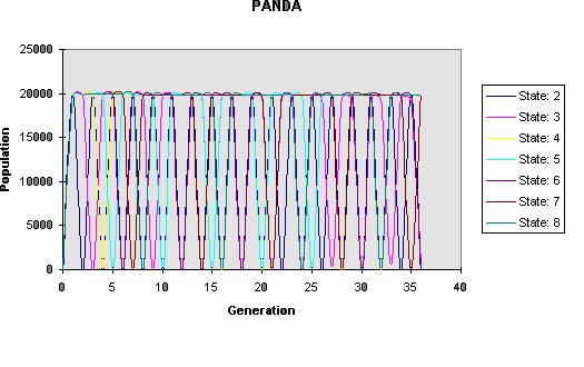
PANDA

data file

(started out with odd population)

Generation	State: 2	State: 3	State: 4	State: 5	State: 6	State: 7	State: 8
0	31	31	31	31	31	31	31
1	19831	19852	19852	19852	19852	19852	19852
2	44	19844	19865	19865	19865	19865	19865
3	19831	60	19880	19901	19901	19901	19901
4	44	19812	67	19885	19906	19906	19906
5	19831	19802	19874	77	19890	19911	19911
6	44	84	19846	19873	75	19891	19912
7	19831	19798	19880	19849	19873	77	19891
8	44	19778	65	19883	19846	19873	77
9	19831	108	19880	19875	19871	19847	19873
10	44	19769	19844	80	19869	19871	19847
11	19831	19743	19880	19878	19866	19869	19871
12	44	136	62	19849	59	19873	19869
13	19831	19742	19875	19883	19857	19866	19873
14	44	19698	19841	19875	19837	66	19873
15	19831	173	19873	80	19856	19865	19866
16	44	19712	58	19878	19857	19845	66
17	19831	19640	19872	19848	19856	19871	19865
18	44	223	19840	19884	54	19869	19845
19	19831	19669	19873	19874	19847	19873	19871
20	44	19567	58	81	19831	19866	19869
21	19831	277	19870	19877	19848	66	19873
22	44	19630	19838	19844	19850	19865	19873
23	19831	19502	19871	19882	19848	19845	19866
24	44	341	58	19870	50	19871	66
25	19831	19575	19870	79	19846	19869	19865
26	44	19427	19838	19877	19831	19873	19845
27	19831	415	19871	19844	19848	19866	19871
28	44	19517	58	19882	19850	66	19869
29	19831	19342	19870	19870	19848	19865	19873
30	44	499	19838	79	50	19845	19873
31	19831	19456	19871	19877	19846	19871	19866
32	44	19259	58	19844	19831	19869	66
33	19831	584	19870	19882	19848	19873	19865
34	44	19392	19838	19870	19850	19866	19845
35	19831	19163	19871	79	19848	66	19871
36	44	679	58	19877	50	19865	19869

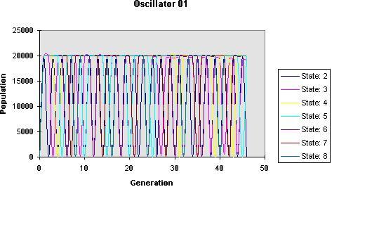
Oscillator 01

data file

(started out with even population)

Generation	State: 2	State: 3	State: 4	State: 5	State: 6	State: 7	State: 8
0	22	22	22	22	22	22	22
1	19935	19957	19957	19957	19957	19957	19957
2	33	19946	19968	19968	19968	19968	19968
3	19935	35	19968	19990	19990	19990	19990
4	33	19928	42	19969	19991	19991	19991
5	19935	19915	19973	61	19976	19998	19998
6	33	56	19955	19977	51	19976	19998
7	19935	19903	19981	19965	19972	61	19976
8	33	19882	39	19992	19970	19982	61
9	19935	81	19988	19965	19974	19970	19982
10	33	19861	19954	65	19981	19992	19970
11	19935	19854	19992	19982	19971	19985	19992
12	33	111	39	19965	60	19992	19985
13	19935	19822	19992	19992	19955	19972	19992
14	33	19815	19954	19965	19971	60	19992
15	19935	146	19992	65	19978	19982	19972
16	33	19780	39	19982	19980	19970	60
17	19935	19775	19992	19965	19965	19992	19982
18	33	184	19954	19992	56	19985	19970
19	19935	19733	19992	19965	19952	19992	19992
20	33	19728	39	65	19938	19972	19985
21	19935	209	19992	19982	19960	60	19992
22	33	19692	19954	19965	19956	19982	19992
23	19935	19675	19992	19992	19958	19970	19972
24	33	252	39	19965	44	19992	60
25	19935	19651	19992	65	19956	19985	19982
26	33	19616	19954	19982	19934	19992	19970
27	19935	291	19992	19965	19952	19972	19992
28	33	19594	39	19992	19944	60	19985
29	19935	19553	19992	19965	19944	19982	19992
30	33	19525	19954	65	28	19970	19992
31	19935	19482	39	19982	19938	19992	19972
32	33	405	19992	19965	19922	19985	60
33	19935	19468	19954	19992	19934	19992	19982
34	33	19415	19992	19965	19934	19972	19970
35	19935	464	39	65	19934	60	19992
36	33	19411	19992	19982	26	19982	19985
37	19935	19336	19954	19965	19934	19970	19992
38	33	519	19992	19992	19922	19992	19992
39	19935	19329	39	19965	19934	19985	19972
40	33	19274	19992	65	19934	19992	60
41	19935	587	19954	19982	19934	19972	19982
42	33	19256	19992	19965	26	60	19970
43	19935	19183	39	19992	19934	19982	19992
44	33	664	19992	19965	19922	19970	19985
45	19935	19190	19954	65	19934	19992	19992
46	33	19099	19992	19982	19934	19985	19992

ACORN

data file

(started out with odd population)

Generation	State: 2	State: 3	State: 4	State: 5	State: 6	State: 7	State: 8
0	7	7	7	7	7	7	7
1	19966	19972	19972	19972	19972	19972	19972
2	9	19968	19974	19974	19974	19974	19974
3	19966	19	19981	19987	19987	19987	19987
4	9	19960	18	19983	19989	19989	19989
5	19966	19946	19982	23	19984	19990	19990
6	9	41	19969	19985	24	19986	19992
7	19966	19943	19984	19975	19980	22	19986
8	9	19919	19	19981	19968	19978	22
9	19966	70	19986	19980	19973	19965	19978
10	9	19918	19969	20	19973	19966	19965
11	19966	19887	19986	19980	19970	19966	19966
12	9	109	19	19976	13	19966	19966
13	19966	19889	19986	19980	19971	19966	19966
14	9	19854	19969	19980	19964	8	19966
15	19966	154	19986	21	19967	19966	19966
16	9	19851	19	19980	19967	19963	8
17	19966	19822	19986	19976	19967	19966	19966
18	9	206	19969	19981	9	19966	19963
19	19966	19803	19986	19980	19967	19966	19966
20	9	19792	19	21	19964	19966	19966
21	19966	266	19986	19980	19967	8	19966
22	9	19745	19969	19976	19967	19966	19966
23	19966	19764	19986	19981	19967	19963	19966
24	9	336	19	19980	9	19966	8
25	19966	19679	19986	21	19967	19966	19966
26	9	19736	19969	19980	19964	19966	19963
27	19966	414	19986	19976	19967	19966	19966
28	9	19605	19	19981	19967	8	19966
29	19966	19708	19986	19980	19967	19966	19966
30	9	500	19969	21	9	19963	19966

ANALYSIS:

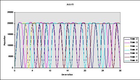
We realized for most of my patterns (JINX, Panda, Oscillator, and Acorn) the states two and four through eight were periodic in nature. Although they are periodic, it is evident that there are boom and bust cycles, with the boom occurring as the population increases, and the bust occurring as the population crashes and decreases. Overall, it is evident on the graph for states two and four through eight that there exists a carrying capacity at around 10,000. The population size oscillates around this number. Altering the states overall had no effect on the carrying capacity. When we altered the states, the carrying capacity continued to occur at around 10,000. The difference was that when the states increased, the population was maintained at a larger population for a longer period of time.

Overall, we saw that the number of states equaled the number of generations in a cycle (i.e. the fifth state had five generations within a cycle) except State 3 on all and the fourth state on JINX. State three graphs showed a regression of the maximums and minimums; therefore the graph decreased vertically in size. The trend eventually narrowed down to a range within the 5000s. Thus, the carrying capacity was around this number.

So, we analyzed the third state more closely. Since the behavior of the third state was the same for all four patterns, we decided a concentration on one would prove necessary. We decided to study JINX.

The graph below represents the population numbers which were low, and it focuses on what kind of cycle they are in. Based on the graph, at first it looks as if the numbers increase exponentially. We ran the pattern until around the 600^th generation and found that the population averaged out around 5000-5300. Therefore, this graph would start out exponentially, but at a certain inflection point, it changes and becomes more logistic, reaching a limit. This would support the logistic growth of populations found in populations, where the population of an organism reaches some limit. This limit that the population is influenced by is the carrying capacity, the number of individuals the environment can support for a certain amount of time. Time, in this instance, is represented by the number of generations. The carrying capacity may be influenced by the food supply or access to sheltered sites (in animals), or access to sunlight or the availability of water (in plants). In the third state, it just so happens that the carrying capacity occurs at around 5000-5300.

The following graph represents the high population figures within the same pattern JINX. Unlike the graph above, it decreases exponentially, and then at some inflection point (not represented on graph), the exponential graph evolves into a logistic graph, in which the population reaches some limit. However, in the following graph, it is different from the one above because unlike the one above, the graph does not increase until it reaches a carrying capacity. Instead, it decreases until it reaches a point where the population is henceforth stabilized between 5000 and 5300. This population is obviously influenced by the carrying capacity though, since it approaches a limit and the carrying capacity represents the limit where the population is maintained. So, even though the population numbers are decreasing, they are approaching a number that the environment can provide for, the carrying capacity. Thus, in both graphs, the curves started out exponential, but later emerged as logistic, showing that the population was influenced by the carrying capacity in the third state.

The following graph is an overall graph of the population numbers recorded from the 1434 to the 1490 generation. The graph shows that the graph oscillates around 5000-5300. Although the population numbers have changed drastically from the beginning thirty generations, Jinx has still retained the periodic cycle. It has merely evened out around a certain population (represented by this carrying capacity). Although the population still hasn’t emerged as a repetitious cycle (and it’s likely it never will), it does act as an oscillating pattern influenced by the carrying capacity.

Overall, we did not encounter much uncertainty since the data we obtained came exactly from the cellular automata program. However, it is possible, that as we recorded the data into Excel, we accidentally entered inaccurate data. Also, CAV (cellular automata viewer) and cellular automata in general are relatively new, and there may be certain concepts that have yet to be discovered about the program.

Back to Top

DISCUSSION/CONCLUSION:

Our data proved my hypothesis to be correct. In our hypothesis, we predicted that the number of generations in a repeating cycle would increase as we increased the number of states.

For example:

2^nd state: 19831, 44

3^rd state: never emerged as a repetitious cycle

4^th state: 58, 19870, 19838, 19871

5^th state: 19877, 19844, 19882, 19870, 79

6^th state: 19831, 19848, 19850, 19848, 50, 19846

7^th state: 19871, 19869, 19873, 19866, 66, 19865, 19845

8^th state: 19871, 19869, 19873, 19873, 19866, 66, 19865, 19845

Not only did it increase, but the number of generations in a cycle equaled the number of states. This was evident in the above examples (taken from Panda’s data). All of this occurred in each trial (Panda, JINX, Acorn, Oscillator 1) except with three, and state four did not work in JINX. We do not know why three didn’t work, but it never emerged as a cyclic pattern. Although it did look periodic, it just wasn’t a repetitive cycle. In the third state, the low populations steadily increased and the high populations steadily decreased, so eventually, the population stabilized around 5000-5300. This occurred around the 600^th generation. We could have made our lab more accurate by actually tracking the data points at these generations (from the first generation to the 1500 generation) and depicting this information on a graph, but that would have been over ambitious. Instead, we found it sufficient enough to graph the beginning thirty generations, and then the 1434-1490 generations, just to show what the population eventually looked like. We figured by just eyeing the population numbers at the 600^th generation, we would have been led to the same conclusion. Also, we do not really know why state four did not work in JINX. However, state four wasn’t nearly as random as state three for although it did not follow the same pattern as the other states, it did operate around the same numbers, just not exactly. In states three and four, the populations did cycle in the same fashion, where the number of generations in the so-called pattern did equal the number of states; however, these numbers were not exact. And state three eventually led to a different population of 5000-5300, whereas state four basically stayed around the same population. Thus, although not all of our data supported our hypothesis, the vast majority of it did. An additional hypothesis that might have explained my data could have been that the number of generations within a repetitious cycle would equal the exact number of states which the pattern was in. In all of our population graphs, we were able to observe there being a carrying capacity that influenced the population. For states two and four through eight, this carrying capacity seemed to be around ten thousand, even though the graph wasn’t necessarily logistic. The graph was stationed around this carrying capacity and would increase or decrease, but it oscillated around this point. The graph of the third state also proved to have a carrying capacity, despite its randomness. After examining the high and low population numbers, we discovered that the graph eventually emerged as a logistic graph, with a carrying capacity of around 5000-5200. Overall, the graphs for state two and four through eight contained repetitious cycles, which are not truly common in actual life. Therefore, perhaps state three was a more accurate predictor of actual life patterns due to its randomness.

As was stated before, in life-like behavior, the automata behave in ways like those of biological systems. The cells may: “die out, become stable or cycle with a fixed period, grow indefinitely at a fixed speed, or grow and contract irregularly” (Green). Our data possessed this life-like behavior, characteristic of biological systems. In states two and four through eight the cells emerged as a pattern that became stable and cycled with a fixed period. Likewise, in state three, the cells grew and contracted irregularly, while at the same time, they eventually became stable. So even though this was a computer program, it was able to emulate what actually occurs in nature, the interaction between organisms (cells), and the effect of the states (environmental factors like topography) on their population. The program also produced populations whose populations were reminiscent of population trends that occur in nature, as well as populations that possessed carrying capacities, which are evident in nature.

Overall, our method was effective in producing the results we wanted. Some limitations we encountered were present in the actual cellular automata program we used. For instance, a limitation could have been the number of states that we could alter. We could only alter the states from two to eight. We do not know if there exists a program in which more states can be altered, but if such a program exists, it would have allowed us to study the effects of altering the states more extensively. Also, another limitation could have been that we only emphasized the importance of the states. We could have researched the effects of altering all of the parameters, including the birth and survival rate. Instead of having the birth and survival rate at zero all the time, we could have changed it to one for both the survival and birth rate. However, it would have taken years to analyze and compile all of the different combinations. Also, it might have been better if we had examined a different birth and survival rate since zero is a bizarre number to have as the birth and survival rate. Having zero as the birth and survival rate would mean that in order for a cell to survive, it must have zero neighbors, and for a cell to be reactivated, or born, it must have zero numbers. This combination would not occur in nature, since in order to survive, or “reproduce,” it is necessary to have neighbors. Thus, having zero has the birth and survival rates at zero could have been an unrealistic combination and one that is unrepresentative of what actually occurs in nature. It would almost be like spontaneous generation in a sense, since a cell would be born without needing any neighboring cells. Instead of cells reproducing, a cell would just suddenly appear out of nowhere, much like in spontaneous generation.

Also, we could have researched the other programs within the cellular automata viewer, which would have included vote mode, mode 1D (Wolfram), and mode 1DB (Langton). However, we knew beforehand that we wanted to research the life program because we would be able to alter the parameters more easily. Plus we did not have enough time to do a comprehensive study of everything in the cellular automata viewer. It was realistic to emphasize a quality about a particular mode, and go in depth about the effects that quality has on the mode. This was exactly what we did: we specifically studied the life mode, and researched the effects of altering the states. Since we always had the birth and survival rates at zero, we were able to do an in-depth study of one environment. Also, we could always have done more patterns, but we found that four patterns were sufficient enough. Also, we could have collected more data points for each pattern, especially for the third state. Since we stopped at around thirty to forty generations, we never closely examined what the population size was at the 600^th generation. We did, however, run it, and we made assumptions about what eventually occurred. If we wanted to make an improvement, we could have collected population numbers for the third sate when it’s generation number was really high (continued after the 1500 generation). We could have done this for the third state in each pattern (Jinx, panda, Oscillator 01, and Acorn ). Instead of analyzing all the pattern’s third state, we just examined Jinx’s. We had noticed that the third states had behaved pretty uniformly; however, there could have been subtle differences that might have altered our conclusions about the third sate. Thus, we could have gone more in depth on the third state for all four patterns, instead of just one.

Bibliography

Ehrencrona, Andreas. Cellular Automata. 28 Oct 2002 <http://cgi.student.nada.kth.se/cgi-bin/d95-aeh/get/lifeeng>.

Evolving Cellular Automata. 2000. EvCA Group. 28 Oct 2002 <http://www.santafe.edu/projects/evca/>.

Green, David G. Cellular Automata. 1993. Charles Sturt University. 28 Oct 2002 <http://life.csu.edu.au/complex/tutorials/tutorial1.html>.

Preston, Kendall Jr., and Michael J.B. Duff. Modern Cellular Automata: Theory and Applications. New York: Plenum Press, 1984.

Wojtowicz, Mirek, ed. What is Life and Cellular Automata?. 07 Jan 2002. Mcell. 29 Oct 2002

<http://psoup.math.wisc.edu/mcell/whatis_life.html>.

Wolfram, Stephen. Cellular Automata and Complexity: Collected Papers. 2002. Stephen Wolfram, LLC. 28 Oct 2002

<http://www.stephenwolfram.com/publications/books/ca-reprint/>.

Wolfram, Stephen. Theory and Applications of Cellular Automata (including selected papers 1983-1986). Singapore: World Scientific

Publishing, 1986.