The Effects of Force and Friction with a Constant Velocity
Background Intentions in the Investigation Preparation Work Procedure Investigational Variables Presumptions Within the Experiment and Set Up Assembling Data Graphed Data Uncertainty Values of Time Improvement Upon Experiment Overall View of Experiment Related Links Return to Research
Background Go Up
Without friction in the world, objects would continue to move stating Newton’s First Law of Motion: an item will persist in a fixed motion in a linear direction until another force interrupts its inertia. This fascinating principle of physics was discovered by Sir Isaac Newton because he understood that in it necessary is for everyday life to maintain firmness from gliding constantly on a surface.
In order to gain this state of motion, there are two scenarios: an object is at rest and stays at rest, or an object is in motion and continues in that constant motion. However, with Newton’s Second Law, it applies that to any difference in the movement, a new force is applied that results to the object either accelerating or decelerating. The forces that are commonly applied in Newton’s Second Law are: reaction force, dynamic force, gravity force, and friction force.
Intentions in the Investigation Go Up
The motive to conduct the investigation is to test Newton’s Laws. The most efficient to organize it is to have it carried out in an environment where I have the most in control with as many variables, to find out whether his principles are true on a smaller scale familiar in common environments. Which is why I chose two different environments: a dry rug in room temperature, and wet grass in cold climate when the research began. Furthermore, to observe the relationship between how a constant velocity may have any effect on force and force of friction.
For my hypothesis, I believe that with a constant velocity, the forces that are acting on the object will stay at a constant rate since from Newton’s 2nd Law of Motion. Where there is no other force being introduced; therefore it is not accelerating or decelerating. Even with trying different surfaces, it should apply to all of them. Therefore, when placing the number of newtons that the forces are acting upon on a graph for distance and time, it should look like a stagnant line as if it were to continue to infinity.
Preparation Work and Set Up Go Up
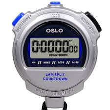
Digital Stopwatch: It is preferable using a stopwatch to measure how long it takes the car to go the distance because mechanical ones would be difficult to read. Adding more human error to the experiment.
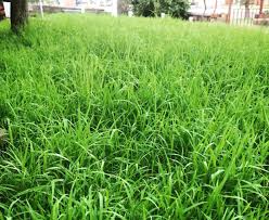
Surface Areas: To understand if constant velocity affects the forces around the moving object, it is necessary to see if any outside interference will make any difference. For that reason, choosing two opposite surface areas will give better results to see if a dry surface area has any effects on forces compared to a wet one. Therefore, the two surface areas I chose to have the car moving on is a regular flat rug and flat grass field.
It is important that these areas are flat because since the point of the experiment is if the constant velocity has any effect on forces, which is why it is necessary the velocity is not speeding up or slowing down. It is required that the velocity be constant in order for this experiment to be a success.

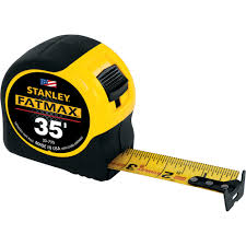
Meter Sticks/Measuring Tape: Without a tool to measure the distance that the car needs to go, it would very difficult to get an accurate measurement. As well as, since the measuring tape failed to fully get to the intentional 5 meters to do the experiment, it was obligatory to add meter sticks to assist in the measurements. Without these tools, I would not have been able to have an array of distances to observes efficiently the relationship between constant velocity and forces on an object
Remote-Control Car: This is the most effective and crucial part of the examination is seeking out an item such as this that had the ability to go at a constant rate. A regular car would suffice since the much human error would occur with the gas pedal; therefore, had to think much smaller for this. A remote control car would suffice because as holding the trigger to keep the car going was only part that matter for it to move forward. As well as, since it had two different speeds (high and low speed), this also gave me more to work with because I could discover whether the pace of the speed mattered in the relationship with the forces.
Before the experiment has started, I give it a test drive to make sure it does not have any flukes or mechanical problems within the car to get sufficient data. As well as, if it can go on the surfaces well and smoothly without any interruptions with its inertia.
Procedure Go Up
To conduct the examination, the necessary tools I would apply to gather data are the stopwatch, two different surface areas, meter sticks, and finally the remote-controlled car. I set up a linear path the car can take by placing the meter stick and measuring tape to the side of the car, which will ensure a direct path for it to take. Then afterward I would place the car’s front wheels right at the zero marks of the meter stick/measuring tape to ensure it does not start at the one mark to get accurate measurements.
Right as the remote control car is about to go at a sustained pace, I will have a stopwatch to time how far it takes to go the certain distance I want it to go. I repeat this procedure five times with the two different speeds (high and low speed) on both of the dry and wet surface areas to be certain I get a wide variety of outcomes.
Investigational Variables Go Up
One of the constant variables in the experiment was the weight of the car, which was 3.72 kg. This is the most critical information because it is a major factor in several of the equations I will use. As well as, the surface areas because I utilized the same areas where I drove the car. This was crucial to gather the data for it to be feasible, which is why I recorded all of them at the same spot of the surface areas. Additionally, the coefficient of friction is worthy to discuss since they are the key element of the equations to determine the force and force of friction. Since I only focused on two surface areas, only two coefficients of friction I am able to focus on.
First off, the independent variable I have the most control over was the distance. I chose five different distances (measured in m) that were easy to follow in order to time it correctly when the car finally accomplished passing it. Having different distances for the car to go along, it gave an opportunity to observe of variety data I would receive. Furthermore, the speed of the car I am able to manipulate since it has the ability to perform two different speeds. This will be efficient since it can either approve Newton’s Laws. Or disprove Newton’s principles of motion if there is a certain speed necessary that will cause the forces to act differently.
The dependent variable most vital within the experiment is certainly time. With this, I can succeedingly calculate the acceleration by using SUVAT, meaning the acronyms within it represent the variables: s = displacement, u = initial velocity, v = final velocity, a = acceleration and t = time. Additionally, once I have obtained the acceleration for each distance the object has done, the forces (measured in newtons) around the object while it is at a sustained pace, will be constructed using the formulas: Ff= uF for force of friction, and F=ma to find specifically the dynamic for acting upon it.
Presumptions Within the Experiment Go Up
1. It is reasonable to assume that as more distance is traveled, it will take more time to reach the destination as is shown in Graph 1 and Graph 2.
2. The reaction and gravity forces that push on the object is assumed as they are in mathematics process, but they cancel each other out. As well as they will not be considered during the experiment since they do not have an effect while an object is moving horizontally. Therefore, they are as well considered constants while the car is in a sustained motion.
.png)
Graph 1
Graph 2
Assembling Data Go Up
|
Dry Surface Area Times (s) |
1 |
2 |
3 |
4 |
5 |
|
High Velocity |
0.46 |
1.7 |
1.98 |
2.54 |
3.46 |
|
0.68 |
1.28 |
2.06 |
2.58 |
3.28 |
|
|
0.58 |
1.19 |
1.96 |
2.63 |
3.37 |
|
|
0.61 |
1.26 |
1.99 |
2.67 |
3.41 |
|
|
0.67 |
1.07 |
2.01 |
2.88 |
3.13 |
|
Dry Surface Area Times (s) |
1 |
2 |
3 |
4 |
5 |
|
Low Velocity |
0.85 |
2.17 |
3.08 |
4.35 |
5.41 |
|
|
1.19 |
2.28 |
3.39 |
4.44 |
5.6 |
|
|
1.18 |
2.23 |
3.36 |
4.5 |
5.59 |
|
|
1.12 |
2.25 |
3.29 |
4.45 |
5.53 |
|
|
1.16 |
2.07 |
3.43 |
4.31 |
5.47 |
Figure 1
|
Wet Surface Area Times (s) |
1 |
2 |
3 |
4 |
5 |
|
High Velocity |
0.36 |
0.78 |
1.47 |
1.77 |
2.13 |
|
|
0.57 |
0.92 |
1.41 |
1.92 |
2.27 |
|
|
0.41 |
0.88 |
1.28 |
1.76 |
2.47 |
|
|
0.43 |
1.05 |
1.35 |
1.87 |
2.3 |
|
|
0.53 |
1.02 |
1.44 |
1.98 |
2.43 |
|
Wet Surface Area Times (s) |
1 |
2 |
3 |
4 |
5 |
|
Low Speed |
0.54 |
1.38 |
1.92 |
2.38 |
3.13 |
|
|
0.67 |
1.26 |
1.84 |
2.58 |
2.84 |
|
|
0.62 |
1.22 |
1.95 |
2.43 |
3.21 |
|
|
0.58 |
1.19 |
1.77 |
2.48 |
3.26 |
|
|
1.2 |
1.89 |
2.63 |
2.71 |
3.18 |
Figure 2
As it is presented in Figure 1 and Figure 2, these are the times (in seconds) collected for each distance (measured in meters) the car has completed going through. These were all completed by observing the car as it drove the certain distance and timing it the latest it passed. For the calculations, I will use the average times. By obtaining the average time, I will have added all them per column and divided it by five.
Graphed Data Go Up
Similarly to what we have seen in Graph 1 and Graph 2, those are the averages from each column for each distance. As it was previously mentioned, it is assumed that as distance continues to grow, it would take longer to get there. By using the average times, they would be utilized in the equations by SUVAT: a=1/(t(v-u)) in order to find acceleration. Here is an example of how the formulas would be used from the data of the High Speed from Dry Surface Area. a= 1/(0.6(3m/s-0m/s))=4.5m/s/s. With the formula, I was able to create a graph with all the calculated accelerations.
Graph 3
Graph 4
These graphs illustrate the relationship between distance and acceleration. As it is demonstrated, it is seen as if the acceleration as distance continues, it declines very quickly. Therefore, there is a limit it reaches because as velocity is constant, there is no other way it can increase or decrease. Then will continue in the stagnant acceleration it is until the velocity has changed.
Now that the acceleration has been discovered through SUVAT, to find the Dynamic Force, the equation: F=ma will not be applied. Here is an example of using the formula by using mass of the car and the acceleration of Slow Velocity from Wet Surface: F=(3.27kg)(9.24m/s/s)=34.4N.
Graph 5
Graph 6
Uniformly such as the previous graphs of acceleration, dynamic force as well reaches a certain point of limitation as distance continues. Because there are no other forces being added on to the car as a sustained velocity continues, there is no high nor low curves on the graph. It looks more like exponential as it continues for five meters.
Finally, now having finished calculating the dynamic force for each distance, it will be used to calculate the friction force with the equation of: Ff=uF where u is the coefficient of friction of friction for every surface area possibly imagined. For every surface area, there is a coefficient of friction. Here is an example of the equation by using the force from Dry Surface Area with High Velocity: Ff=(.20)(1674N)=3.35N.
Graph 7
Graph 8
Identical shape the graphs have as the previous graphs shown with the relationship with distance. As the distance continues, there will be the limit to how much force of friction it is restricting the car’s movement. Therefore, as there is no new velocity, acceleration, or dynamic force acting upon the object, the force of friction will become stagnant. The best-fit lines demonstrate clearly that the relationship with distance is a steadily decreasing and motionless limit.
Uncertainty Values for Time Go Up
Since the values of acceleration, dynamic force, and force of friction are purely calculations, they are all affected by time which what should more focused on to determine uncertainty. By utilizing the formula: change of t=(tmax-tmin)/2 for each value in the data for time per distance.
|
Dry Surface Area Times (s) |
1 |
2 |
3 |
4 |
5 |
|
High Velocity |
0.6+/-0.1 |
1.3+/-0.6 |
2.0 +/-0.5 |
2.7+/-1.0 |
3.3+/-0.2 |
|
Dry Surface Area Times (s) |
1 |
2 |
3 |
4 |
5 |
|
Low Velocity |
1.1+/-0.2 |
2.2+/-0.2 |
3.3+/-0.2 |
4.4+/-0.1 |
5.3+/-0.2 |
|
Wet Surface Area Times (s) |
1 |
2 |
3 |
4 |
5 |
|
High Velocity |
0.5+/-0.1 |
1.0+/-0.5 |
1.4+/0.2 |
1.9+/-0.2 |
2.3+/-0.3 |
|
Wet Surface Area Times (s) |
1 |
2 |
3 |
4 |
5 |
|
Low Speed |
0.6+/-0.7 |
1.3+/-0.7 |
1.9+/0.9 |
3.0+/-0.3 |
3.1+/-0.2 |
Here it illustrates near the times for Dry Surface Area and the first Wet Surface Area for High Velocity, the uncertainties were fairly low because the times were able to be precise with a stopwatch. However, by the last Wet Surface Area for the Low Velocity, the uncertainties were very scattered because since it was difficult to determine when it surpassed the distance.
Improvement Upon Experiment Go Up
One of the errors with the project that can be determined is the flaws of the items that I used. The measuring tape and meter sticks that are placed along the car to determine its path, may not have been correctly 1m, 2m, etc. There must have been a human error when measuring the distances. As well as the car because since it is remote controlled and relies on an antenna to cooperate, I may have been too far from it in order to make sure it kept a sustainable pace. Furthermore, the surface areas I utilized may not have been completely flat for the car, but for the person, it may appear that it is flat. Should have determined more closely if they were any dips or bumps in the path that was taken
Environmental errors were also taken in place because the weather would also have an impact on the car if it was raining, compared to if it were sunny. It could have impacted the speed of the car. Additionally, air friction could be taken accounted for because it is the one variable that is uncontrollable; therefore consider it a constant.
Perceiving when the car passed the finish line is also an action conducted that has human error. As well as a human error with the timer since it may take a while for the person to react to the car finishing the distance
Overall View of Experiment Go Up
It was an exciting procedure to conduct since it would give me an opportunity to have in control of what I want to see in Newton’s principles of motion. The experiment showed me what errors I should improve on to better future explorations within science or any other topic. As well as approving Newton’s First Law of Motion that it will keep at the same pace until a new force is introduced.
So in my conclusion with this, it does not matter the surface area being used to express Newton’s First and/or Newton’s Second Law of Motion because it applies to all. Additionally, the relationship of velocity with forces is that as velocity continues, the forces will reach a limit of how much it is put surrounding the car as distance continues.
1. Crash Course Video on Friction: https://www.youtube.com/watch?v=fo_pmp5rtzo&t=87s It was a formal demonstration of how friction worked on surfaces.
2. Types of Forces: https://www.physicsclassroom.com/class/newtlaws/Lesson-2/Types-of-Forces A written document that represented and illustrated the different forces acted on an object.
3. Newton’s Laws: https://www.grc.nasa.gov/www/k-12/airplane/newton.html Describing the different laws he has and created.
4. Newton’s Second Law: https://www.grc.nasa.gov/www/k-12/airplane/newton2.html Illustrates the second law and how it impacts everyday objects
5. Gravity, Force, and Work (Clip): https://www.youtube.com/watch?v=LEs9J2IQIZY A less formal demonstration on when gravity and work is put into play on the object itself.