How does distance affect the intensity of light?
Table of Contents
Procedure | Data
| Calculations | Graph
| Analysis | Changes
to Lab | Go Up
Introduction:
Johannes Kepler, renowned German mathematician and astronomer, described the effect of gravity as a direct proportion to the inverse of the distance between the two objects. However, in 1645, a French astronomer named Ismaël Bullialdus corrected Kepler by showing the relationship to actually be proportionate to the inverse of the distance squared. He was essentially showing a geometric dilution from a point source of radiation. The inverse square law also pops up in a very important field of study known as QED, or quantum electrodynamics. QED describes how light and matter interact, and is the first theory that fully reconciles quantum mechanics and special relativity. QED calls for the upholding of the inverse square law with reference to light because photons have a vanishing pole mass. The prediction holds with other massless particles, and explains the inverse square law of gravitational force. Newton also dabbled with the Inverse Square Law in his study of gravity, where he measured the periods and diameters of the orbits of Jupiter and Saturn. He found that the forces on Jupiter and Saturn, exerted by the sun, were proportional to the inverse of the distance squared. Although the inverse square law applies to sound, gravity, and electric fields, Bullialdus focused on light to test this theory. He did this by showing that the intensity of light (I) at a given distance from the origin of the light was the power output of the light source (S) was proportional to inverse of the squared distance. This did not only explain that light decreases over a distance, common knowledge at the time, but that it decreases at a specific proportion to the inverse of the distance squared. Simple geometry can tell us the proportion to be divided by, within the inverse square, is the surface area of a sphere at a given distance (4πr²);
I=S4πr²
This works because the Power output of the light source has to be divided by the surface area it has to cover. If the intensity was measured one meter away from the light source, the intensity would be the power (S) divided by 4π times 1 squared. This makes the intensity of light proportional, the proportion is 1/(4π), to the inverse of the distance squared.
Hypothesis:
If I measure the intensity of light at a given distance of r, it will decrease proportionally to the inverse of the distance squared.
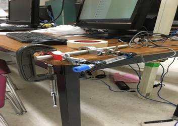
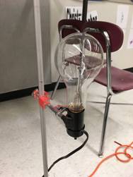
Design:
I intend to test this by illuminating a 150 Watt Tungsten Incandescent light bulb in a dark room and testing the intensity of the light at many different distances. I am going to increase the distance and record the intensity of light. My aim in this investigation determine whether the intensity of light decreases as a proportion of the inverse of the distance squared, and I hypothesise that the real-world results will reconcile with the math.
Materials
150W
Tungsten light bulb
Vernier Light Sensor
Various
clamps for holding sensor and light bulb
Computer
with LoggerPro
Tape
measure for measuring length and height
Procedure
Back to top
Set
up lab area, including computer, sensor, and light bulb.
Turn
off all sources of light in room.
Measure
and record the distance between the light source and light bulb.
Take
data for 1 second, then record the value.
Repeat
steps 3 and 4 for varying distances from the light source.
Once
data is all taken, run data through calculations to represent intensity of the
light in Watts per square meter.
Plot
data, once to show inverse square curve, and once to
show linearized data.
Diagram
Variables:
Independent Variable: Distance
I am going to be incrementally increasing the distance between the light source and the fixed light sensor to get a smooth graph showing the 1/r2 relationship.
Dependent Variable: Intensity of Light
I am measuring the intensity of light using a fixed light sensor.
Controls: ambient light in the room, wattage of bulb, increment of measurement, reflective surfaces in the room, reflective potential of my body, angle of lightbulb, height of lightbulb.
Data Back to
top
|
Distance (m) |
Intensity (Lux) |
Intensity (W/m^2) |
Expected |
|
0.23 |
280.23 |
234.762 |
225.645 |
|
0.25 |
245.297556 |
205.4 |
190.986 |
|
0.3 |
163.53170403 |
137.14 |
132.629 |
|
0.35 |
120.27241607 |
100.76 |
97.442 |
|
0.4 |
92.352142525 |
77.37 |
74.604 |
|
0.45 |
72.739703621 |
60.95 |
58.946 |
|
0.5 |
58.37007538 |
48.9 |
47.746 |
|
.6 |
40.929346198 |
34.29 |
33.157 |
|
0.75 |
26.1411994 |
21.9 |
21.221 |
|
.9 |
18.417763692 |
15.43 |
14.737 |
|
1 |
14.92077592 |
12.50 |
11.937 |
|
1.25 |
9.588687434 |
8.033 |
7.639 |
|
1.5 |
6.340732933 |
5.312 |
5.305 |
|
1.75 |
4.880884217 |
4.089 |
3.8977 |
|
2 |
3.59292284 |
3.01 |
2.9842 |
|
2.25 |
3.0402573 |
2.547 |
2.3579 |
|
2.5 |
2.466105843 |
2.066 |
1.9099 |
|
2.75 |
1.914633965 |
1.604 |
1.5784 |
|
3 |
1.595926192 |
1.337 |
1.3263 |
|
3.25 |
1.383454343 |
1.158 |
1.1301 |
|
3.5 |
1.20321137 |
1.008 |
0.9744 |
|
3.75 |
1.067133894 |
0.894 |
0.8488 |
|
4 |
0.9346374033 |
0.783 |
0.746 |
|
4.25 |
0.8260141547 |
0.692 |
0.6609 |
|
4.5 |
0.7317148509 |
0.613 |
0.5895 |
|
4.75 |
0.6541268161 |
0.548 |
0.5291 |
|
5 |
0.5932500504 |
0.497 |
0.4775 |
Calculations
Back to Top
I had to use multiple conversions and calculations to reconcile my data. The sensor measured the luminous flux per square meter in Lux, which equals one lumen per square meter. The best way to represent this data is in watts per meter squared;
I=E x Aη x m² = I=E x 4πη
Where the Intensity, in Watts / m², is equal to the Illuminance, in Lux, times the surface area, in m², divided by the luminous efficacy, in Lumens / Watt, times the squared distance, in m². It can be simplified by removing the distance squared and leaving the 4πin the numerator.
As an example, for the 1.5 meter reading,
I=6.34 x 4π15, I=5.312
For the Expected Values shown above, the equation
I=1504πr²
was used to give a mathematical approximation for the target value of my experiment.
Error; I took the difference between my calculated and measured data, and divided that by the calculated data to get a value for the percent error.
Error=100 x |expected-measured|/measured
I calculated error for all my data points and averaged them to get ~3.9% error.
Graphs
Back to top
Y as a function of X
Analysis
Back to top
The data I measured was very accurate. It shows a direct correlation to the hyperbolic graph of 1/r2, and follows the trend all the way down, I calculated the error present in my data and got a relatively low value of 3.9%. The practice of the inverse square is extremely similar to the theoretical. It holds well in the middle of the spectrum, but grows less practical towards the extremes. If you were to get infinitely close to a light source it would be infinitely intense, which is not feasible to measure.
However, when I linearize my data, and graph Y as a function of 1/X^2, it is a lot more compelling. In a perfect world, my data would produce a perfect line, and the r^2 value is incredibly close to 1. This supports my experiment and my data by showing a very direct correlation between my data and a perfect line. It shows that I was very accurate in replicating the inverse square law
Conclusion
I was successful in testing and affirming the Inverse Square Law with reference to Light. The data I collected was decently accurate, ~3.9% error, and reflected a hyperbolic trend proportional to 1/r2. The linearized graph helped to strengthen my data and my procedure, and provides an easy way to assess the accuracy of my data. My data affirmed my hypothesis in that the intensity of light did decrease at the projected rate, very close to an exact trend.
Errors and
Limitations
Although my data was decently accurate, there were a few key sources of error. All of my measured values were slightly higher than those calculated through the equation, and I think reflected light is to blame for this. I used the large, darkened physics classroom at my school to gather data. For the most part, barring the occasional printer light or computer power button, there were no external light sources present. However, there was certainly potential for reflected light to find its way into the light sensor. The floor of the room is linoleum, which certainly reflected some of the light, as well as metal tables and chairs around the room. I think this was the most significant factor in the error in my lab, skewing all my data high.
. Another thing to discuss is the human error present in the lab. I hand measured the distances between the bulb and the sensor, and it is impossible to be exact in these measurements. Even though I don’t think human error made a significant impact in the volatility of my data, it has to be mentioned.
The third potential source of error in my lab was the imperfections of the light bulb and sensor. I used an incandescent light bulb in my lab, so the origin of the light was not a pinprick, but a small wire. To counteract this, I tried turning the light bulb to find the smallest origin of light with the least resistance. Of course, a true pinpoint of light would be needed to perfect this experiment. The light sensor I used was also not incredibly accurate and required a scaling factor to get a more exact reading. The extrapolation of data within the sensor, as well as potential mechanical inconsistencies could have thrown the data askew.
Changes
to Lab Back to Top
If I were to partake in this lab again, I would make a few key changes. I would get dark, heavy fabric to line the area in an attempt to minimise the chance of ambient or reflected light affecting the amount of light traveling to the sensor. I would also search for a better light source, one that more accurately replicates a point-source of radiation. I would then do multiple trials with different power outputs of light bulbs to see if error increases or decreases as the sheer amount of light increases. The second experiment would focus on eliminating the error I faced in my first experiment to produce more accurate data.
Related Websites
https://en.wikipedia.org/wiki/Luminous_intensity
This Wikipedia page provided useful insight into the concept at play and how they interacted with each other.
http://cse.ssl.berkeley.edu/SegwayEd/lessons/light/measure3.html
A Berkeley lesson on what Light intensity is and how it is changed by amplitude and frequency.
This helps to explain why the inverse square law works with the case of light.
http://hyperphysics.phy-astr.gsu.edu/hbase/Forces/isq.html
Again discusses the inverse square law, but in reference to multiple different fields of application.
https://en.wikipedia.org/wiki/Luminous_flux
Discussion on relations between Luminous Intensity and Luminous Flux.