Gravity cars, despite their simplicity, appear in a shocking number of places, from Pinewood Derby tracks (see Bibliography 1) to the garage of one of Porsche’s Senior Designers (see Bibliography 2). According to a report from the Mechanical Engineering and Mechanical Sciences Department at Duke University, gravity cars are “driven by the force of gravity and must minimize the forces that oppose the vehicle motions, such as wind resistance and friction” (see Bibliography 3). Some such inhibitions are friction created by the axle as it turns and, of course, by drag, also known as air friction or air resistance, which will be discussed below. Usually, as is the case with the Boy Scouts’ famous Pinewood Derby, gravity cars are placed at the top of an incline. The angle that the incline makes with the ground could be variant, as with Pinewood Derby (a steep incline at the beginning followed by a far flatter sections), or it could be an incline plane, in which the angle the plane makes with the ground remains constant, as will be the case in this investigation. The force of gravity on a free falling object (F_g) is (see Bibliography 4):

F_g = mg

F_g is the force of gravity on a free falling object (an object falling directly towards the center of the earth) in Newtons (N).

m is the mass of the object in kilograms (kg). The mass of the car is the only variable that will be directly manipulated in this investigation.
g is the acceleration of freefall at the earth’s surface in meters per second squared (9.81 ms^-2 (see Bibliography 4)); this value will be a constant in this investigation.

However, the force of gravity on an object moving downwards on an incline plane contains a vector component. This equation is (see Bibliography 4):

F_downhill = mgsinθ or F_downhil = F_gsinθ

F_downhill is the downhill force imparted upon the car by gravity, containing the vector component sinθ. The downhill force is expressed in Newtons (N).
θ (lowercase Greek letter theta) is the angle that the incline makes with the ground. The angle of incline will remain constant throughout the investigation.

Of course, the downhill force is only one of the forces acting upon gravity cars. The downhill force is the positive force, the force causing the car to move in the intended direction. The force that this investigation is concerned with analyzing is the force of friction. This force, in contrast with the downhill force of gravity, has many sources. One such uphill force is air resistance, which is generally modelled by the equation (see Bibliography 5,6,7 for comprehensive information):

F_f = -½C_DρAv²

F_f: Force of air friction (N).
ρ: Fluid density (kgm^-3).
A: Cross-sectional area (m²).
v: is the velocity at which the car is travelling (ms^-1).
C_D is the coefficient of drag (unitless, varies with the surface shape and orientation)

This equation might be effective in determining the exact air resistance, but discovering a reliable equation for modelling the other uphill forces, such as friction between the axle and the wheel, is almost impossible; it is simply too nuanced. Terminal Velocity will also play a large role in this investigation. Terminal velocity is the velocity at which the downward force of the object is the same as the upward force. Also, it is the point at which the acceleration is equal to zero. This equation has no inherent use to this investigation in terms of its structure or components. However, the significance of this equation is that it contains a velocity squared component, which suggests that the final formula that this lab will produce will be of degree two.

Return_to_Contents

Problem: Can varying masses of a gravity car and the resulting terminal velocities be used to develop an accurate model for determining the net force of friction?

Hypothesis: By analyzing the terminal velocities of gravity cars with varying masses and comparing each velocity to its respective uphill force, a model for the net force of friction on the gravity car at any velocity can be determined.

Materials:

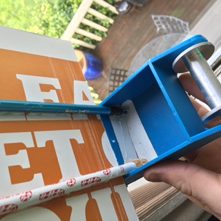
Gravity Car

blue car with trough for weights (provided)
2 popsicle sticks to hold up sail
.04136 m² rectangular poster board sail
hot glue to adhere popsicle sticks to car and sail (see diagram)
set of weights

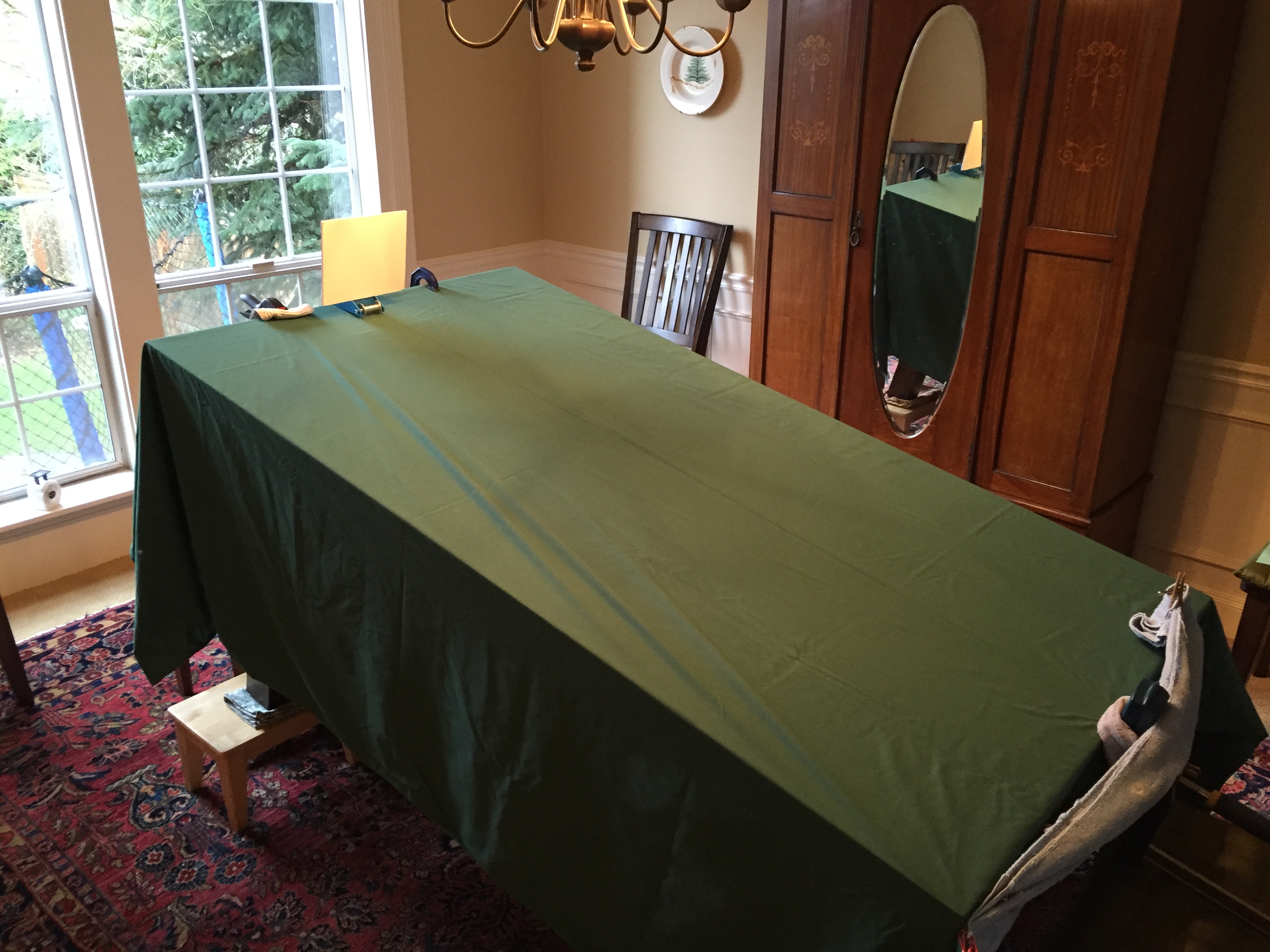
Table (see diagram, dimensions unavailable)
2 identical stools sufficient to prop up table at 11.23 degree angle with the ground
Table cloth to protect surface of table.
Rangefinder
Laptop with Logger Pro
High precision scale
Clamps to adhere rangefinder and table cloth to table.
Tiltmeter app for iPhone 6.

Return_to_Contents

Visuals:

Procedure:

Set up lab area (see Diagram).
Build gravity car (see Gravity_Car).
Download Logger Pro and connect the rangefinder to the computer (via USB).
Use Tiltmeter app for iPhone 6 to measure the incline of the surface.
Put the gravity car, complete with sail, at the top of the incline.
Release the car at the same time as starting the rangefinder recording.
Copy and paste the results up to and including the point at which the car reaches terminal velocity (see Calculations 1 for justification) into a google spreadsheet.
Repeat steps 3 through 5 four times (four trials).
Add 25 grams to the car.
Repeat steps 3 through 7 ten times, so that at the conclusion of the lab there are forty sets of data, four for each of the ten masses.
For each of the 40 sets of data, which should include time, distance, velocity and acceleration, determine terminal velocity (see Calculations 1).
For each of the 10 mass variations, determine the average of the four trials for that specific variation (see Calculations 2). This will give the terminal velocity for that given mass of gravity car. Round to three decimal places (uncertainty is .0005 m/s).
Since each terminal velocity is the point at which the easily calculable downhill force is equal to the infinitely nuanced uphill force, the uphill force (F_U= mgsinθ) can be determined by plugging in the mass that corresponds to the terminal velocity for that data pair (see Calculations 3). Round to three decimal places (uncertainty is .0005 N; the total uncertainty is .001 N).
Plot the force of friction on the y axis of a graph against the terminal velocities on the x axis (see Graph).
Use a calculator or other computational source to find a quadratic model for the data.
Analyze the graph and find the points on the observed data curve that are farthest from the best fit curve. Determine the distance each point’s F_U is from the value predicted by the best-fit quadratic equation. The greatest value will be the uncertainty (which equals the calculated value plus the uncertainty of that value) of the best fit curve.

Return_to_Contents

Data:

Mass (g)	Terminal Velocity (m/s)	Uphill Force (N)	Raw Data Files:
153.5	1.406 ± .001	0.293 ± .0005	Text .:. Excel
179.5	1.430 ± .001	0.343 ± .0005	Text .:. Excel
201.5	1.467 ± .001	0.385 ± .0005	Text .:. Excel
229	1.491 ± .001	0.438 ± .0005	Text .:. Excel
250.5	1.520 ± .001	0.479 ± .0005	Text .:. Excel
272	1.542 ± .001	0.520 ± .0005	Text .:. Excel
298	1.563 ± .001	0.570 ± .0005	Text .:. Excel
323.5	1.601 ± .001	0.618 ± .0005	Text .:. Excel
348	1.623 ± .001	0.665 ± .0005	Text .:. Excel

Additional (371.5g): Text .:. Excel

Graph:

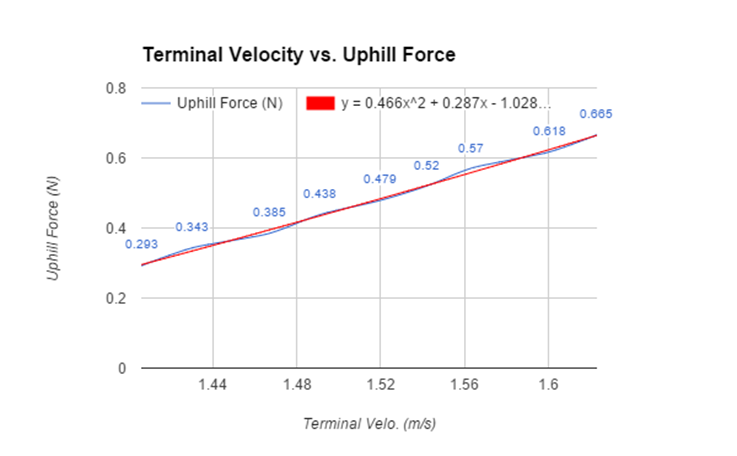
Evaluation: This quadratic equation (F_U = .466V_t² + .287V_t -1.028) modeling the uphill force as a function of terminal velocity will therefore apply for any velocity the gravity car may have at any time*. Therefore, the equation is F_U = .466v² + .287v - 1.028. Of course, there is a .0005 uncertainty in the data for the uphill force and terminal velocities due to rounding, so factoring these into the equation produces the final formula:

F_U = .466v² + .287v - 1.028 ± .013

Return_to_Contents

Conclusion:

Results: The hypothesis was supported, seeing as this investigation was able to determine a degree two polynomial model for uphill force as a function of velocity that adheres very closely to the observed data.

Justification:

Equation: The equation for the force of air friction (F_f = -½C_DρAv²) has a v² component, so I chose a quadratic model based upon the assumption that, since at no time during my research of possible components of F_U(v) formulas did I come across a formula that had a degree other than two or one.

Uncertainty in the data: All data was collected using instruments which operated at the highest degree of precision (with the one exception being the determination of the angle of incline, to be discussed further). The rangefinder, from which all accelerations and velocities (and thus terminal velocities) were determined, returned values accurate to nine or more decimal places. In calculating the terminal velocities (see Calculations 1 and 2), all decimal values were accounted for, meaning that those terminal velocities, in their raw forms, were accurate to nine decimal places as well. Similarly, the masses were determined using a scale which returns a mass in milligrams, one millionth of a kilogram. Thus, when the uphill force at the point of terminal velocity was calculated using F_U= mgsinθ, the uphill force was accurate to six decimal places. Such precision becomes difficult to work with and largely meaningless, considering that each decimal place to left is an entire order of magnitude less significant than the previous decimal place. Thus, in order to produce a concise equation using a uniform number of decimal places for each term, it is logical to round the raw values of terminal velocity and uphill to three decimal places and use proper significant figures later, in the final equation (this will be three significant figures since multiplication is used and the uphill force is three significant figures (see Bibliography 8)). The determination of the angle, however, was accurate only to three decimal places, allowing another .0005 degree uncertainty that cannot be ignored. Since the sine function is being applied on the measured angle, 11.231°, which is very flat angle (that is to say that .0005 will likely skew the value of the sine function by about .0005) has an uncertainty of .0005°, to be added to the uncertainty (of the same value) that comes from rounding to three decimal places. In calculations, the uncertainty value for uphill force and terminal velocity will be, therefore, .001 and .0005, respectively. Ultimately, of course, the final uncertainty will have to match the smallest decimal place of the rest of the equation, three. Each coefficient will be rounded to three decimal places, even though that will mean that the constant term will have four significant figures, for the sake of uniformity.

Uncertainty of F_U in equation: In order to determine the uncertainty of the equation, the maximum deviation in the data from the curve of best fit will be calculated. This will occur at a single point. Thus, the points for which deviation should be calculated are the points that appear to be farthest from the curve of best fit. In analyzing the data (see Data & Graph), the velocities of the points of interest, those which produce uphill forces farthest from the best fit curve are 1.430m/s, 1.467m/s and 1.563m/s (Calculations).

Return_to_Contents

Possible Sources of Error:

Calculations: In order to find the terminal velocity of an individual trial (see Calculations 1), there is likely a small amount of error because in finding where exactly the acceleration was zero was an impossibility. The rangefinder, despite being the best tool available to me, is, of course, imperfect. Therefore, the best way to find the terminal velocity was to find the region where the acceleration was around zero, or the average of the two velocities corresponding to the consecutive positive and negative accelerations. This is an example, first of all, of the limitations of my equipment, and secondly, of my procedure. For the sake of efficiency, I decided on a raw average rather than a weighted one to determine my terminal velocities.

Surface: The surface I used, a tabletop, might have a few ridges or inconsistencies in its surface that might have skewed the data slightly. Also, in starting the car at the top of the ramp, there might have been irregularity in the amount of accidental force imparted in releasing the car. Fortunately, the lag between the release of the car and the starting of the timer would not matter, since all I care about is the data from when the car is about three quarters of the way down the ramp.

The remainder of the errors has previously been discussed in the Justifications section.

Changes to the Lab:

If this lab were to be repeated, I would certainly use a more precise instrument than a free app to measure the angle of incline. I am sure than the gyroscopic sensors in my phone are more than sufficient for the task, but I would still prefer to use more traditional techniques in this instance.

It would be a good idea, too, to use a surface such as the finished plywood composite used in making the tables we use at my school, or some similar material, rather than a dining room table with a sheet over it, in order to achieve a flatter surface.

As is always the case, it would be a good idea to use a greater number of trials or more variation of mass (perhaps add 50g each trial). I decided on 4 iterations of each trial (each mass) because the setup for each iteration took time and each iteration returned consistent results. However, I understand that this is not an optimal number of iteration, so if I had the opportunity to repeat this lab I would certainly add more trials and more iterations of each trial.

For the gravity car, I used a load-carrying car from our physics lab that we have used in class, and I added a sail to it in order to accentuate the uphill force at a point. However, the car, though certainly effective, was constructed haphazardly and I would definitely take the time to construct a more stable design.

Return_to_Contents

Calculations:

To find the terminal velocity for a certain data set, take the velocities from the last instance in which the acceleration is negative (negative because the car is closing in on the rangefinder) and the first instance in which the acceleration is positive. Between these two, there is a moment in which the acceleration was 0, the point of terminal velocity. Average the two to determine the terminal velocity for that specific trial.
To find the terminal velocity for a certain mass variation, simply average the calculated terminal velocity from each of the four trials for that mass variation.
At this point, the masses corresponding to each terminal velocity have been determined. g, the acceleration of gravity, is a constant (9.81) and so too is the angle that the table makes with the ground. Thus, the downhill (and thus uphill) force can be determined by multiplying the mass of a specific variation by the constant gsinθ.

Bibliography:

1. (non-web)

Mann, B. P., M. M. Gibbs and S. M. Sah. “Dynamics of a gravity car race with application to the Pinewood Derby.” Mechanical Sciences (2012) Print.

*The idea of using a gravity car in this investigation came from the novelty of pinewood derby racing. This site provided me with the background on existing analysis of the gravity car conundrum that would provide me the idea for the specific metric that would be measured in this investigation.*

2. http://www.pinewoodderby.org/#/one

"Pinewood Derby." Pinewood Derby. Boy Scouts of America, n.d. Web. 20 Dec. 2015.

3. http://www.tuvie.com/porsche-design-gravity-car-by-3dyn/

"Tuvie." Tuvie Porsche Design Gravity Car by 3dyn Comments. RSS, n.d. Web. 21 Dec. 2015.

4. (non-web)

Physics Data Booklet. Edmonton, AB: Alberta Education, 1985. Web.

*Our own IB Physics Data Booklet was a fabulous source of basic equations which could be combined to derive many of the formulas used in this investigation while staying to the IB format and syntax.*

5. https://www.grc.nasa.gov/www/k-12/airplane/shaped.html

"Shape Effects on Drag." Shape Effects on Drag. NASA, n.d. Web. 21 Dec. 2015.

*This was useful in providing a background for some other ways in which air friction is calculated. For instance, because of the information from this site it was clear that the force of friction is going to be some function of velocity squared.*

6. http://chemistry.about.com/od/gases/f/What-Is-The-Density-Of-Air-At-Stp.htm

"What Is the Density of Air at STP?" About.com Education. About Education, 2 Dec. 2014. Web. 23 Dec. 2015.

*Though I ultimately did not use the given equation for force of friction (it was mostly just there as a point of reference), knowledge of the parent equation and how the units aligned, as given by this source and others, was very interesting and informative and gave the solid background I needed to judge my results authoritatively.

7. http://hyperphysics.phy-astr.gsu.edu/hbase/airfri.html

"Air Friction." HyperPhysics. GSU, n.d. Web.

8. https://www.deanza.edu/faculty/lunaeduardo/pdf/UncertaintyandSignificantFig.pdf

"Significant Figures." AccessScience (n.d.): n. pag. Uncertainties and Significant Figures. De Anza. Web. 28 Dec. 2015.

*Considering that the calculations in this investigation were all multi-step, it became difficult to isolate how the appropriate number of significant figures should be determined. This site provided definitive insight into this process as it is undergone at the college level.*