The Effect of Temperature on the Restitutional Coefficient of a Golf Ball
Introduction
Research Information
This research was conducted in Tualatin, Oregon at Tualatin High School, under the supervision and advice of Mr. Christopher Murray, the IB Physics Instructor. This research project was conceived in October 2013 by Adam Mitchell and Grey Patterson. The data was collected on Friday, 20 December 2013, and the research paper was completed on Sunday, 5 January 2014. Finally, the research defense for this investigation was conducted on Monday, 13 January 2013.
Background Information
The coefficient of restitution is the measurement of the ratio between the initial drop height of an object and the height to which the object returns at the apex of its first bounce in its infinite series of bounces. A perfectly elastic bounce of a ball, in which the ball returns to its original drop height, is defined as the ball having a coefficient of restitution of 1. A collision in which the ball does not bounce after the initial bounce, and immediately lies at rest on the floor, is defined as the ball having a coefficient of restitution of 0 (McGinnis 85). Other definitions and applications of the coefficient of restitution include the measurement of the ratio between the initial velocity of an object and the final velocity of an object during its first bounce; however, these irrelevant applications will not be used in this investigation.
The most common application for the coefficient of restitution, in the modern world, is the area of sports. Golf balls, soccer, balls, footballs, and all sports balls depend on intricate materials and precise manufacturing in order to ensure the respective ball behaves in the desired manner. For example, in the sport of golf, the coefficient of restitution is extremely important, because the sport’s benchmark conditions specify that a golf ball, in “reasonable temperatures”, is to have a coefficient of restitution between 0.800 and 0.900 (Thomas). This standard was created in order to attempt to standardize the frictional, kinetic, and thermal energy loss of the collision between a golf ball and a club. Therefore, the game of golf greatly values the coefficient of restitution, because the aforementioned coefficient has a significant impact on the behavior of the respective athletic ball, and therefore, the outcome of the game.
The one aspect that golf does not account for is whether golf balls can behave differently in different weather and environmental conditions. Because studying the effects of weather and environmental conditions on the behavior of golf ball would involve countless variables and unimaginable amounts of data, this investigation limited itself to studying the effects of temperature on the coefficient of restitution of a golf ball. This, however, encompasses a wide range of potential issues. Firstly, the surface on which the ball bounces has a large impact on the coefficient of restitution (Horwitz and De). Additionally, because the materials of each golf ball are imperfect, each tested golf ball will be slightly different in composition and internal pressure (Calsamiglia and Kennedy). More specifically, Hiroto Kuninaka points out that this investigation must be prepared to account for any factors that impact the law of conservation of momentum (Kuninaka). Different room air temperatures, temperature of the bouncing surface, movement of air particles within the experiment room, and human error will contribute to this experiment’s limitations that this investigation must be prepared to counter in order to ensure the procurement of valid results.
Statement of the Problem and Variables
The purpose of this investigation is to determine the effect that temperature has, if any, on the coefficient of restitution of an athletic ball. Additionally, this investigation will correspondingly answer the question, “at what optimal temperature should a golf ball be dropped in order to produce the highest coefficient of restitution?” In other words, this investigation will attempt to conclude at which temperature a golf ball loses the least amount of energy to an elastic collision.
Statement of the Hypothesis
This investigation believes that the graphical results of this experiment will resemble a bell curve, with the lower temperatures producing relatively low coefficients of restitution, the higher temperatures producing relatively low coefficients of restitution, and the reasonable and moderate temperatures producing relatively higher coefficients of restitutions, because the athletic golf balls were designed for optimal performance in moderate temperatures. This hypothesis is a result of the assumption that the designers of the golf balls attempted to optimize the balls for minimal energy loss at typical temperatures due to the moderate thermal conditions of a game of golf. This investigation furthermore relies on the assumption that the designers of the golf balls did not attempt to reduce the amount of energy lost during an elastic collision at extreme temperatures, because a game of golf is typically not played in extreme thermal conditions.
Method
Experimental Design
This investigation will achieve its aims of determining the effect of temperature on the coefficient of restitution of a golf ball by examining the drop height, return height, and initial temperature of a golf ball over multiple trials. Different golf balls will be used for different temperatures in order to ensure precise results. Additionally, the computerized system LoggerPro will analyze and interpret the drop height and return height in order to eliminate the significant factor of human measurement error.
Materials
The following is a list of materials that were used by this investigation.
- 24 golf balls1
- 5-pound block of dry ice (to cool golf balls)
- 2 1000 ml beakers (to hold water and golf balls)
- 2 hot plates (to heat water)
- 2 temperature probes (to record temperature)
- 1 computer with LoggerPro (to record readings of temperature probes)
- 1 faucet / sink (to procure water)
- 1 hammer (to break dry ice block)
- 2 gloves (to handle dry ice block)
- 1 pair of forceps (to handle dry ice and golf balls)
- 1 insulated cooler (to preserve dry ice block)
- 1 camera with video capabilities (to record videos to be later analyzed)
- 2 meter sticks (to measure drop and return heights)
Procedure
- Gather the aforementioned materials.
- Place the gloves on the experimenter’s hands.
- Place the dry ice block in the insulated cooler and use the hammer in order to break the ice into reasonably sized pieces.
- Fill each of the 2 1000 ml beakers to 600 ml with water from the faucet.
- Place each of the 2 1000 ml beakers on its own hot plate.
- Connect each hotplate to an electrical outlet and turn on the hotplates.
- Place 1 temperature probe in each of the beakers on the hot plates.
- Connect the temperature probes to the computer and open LoggerPro in order to monitor the temperature of the two beakers.
- Manipulate the heat of the first hot plate in order to bring the temperature of the water in its beaker to 100 ± 1 °C.
- Manipulate the heat of the second hot plate to 73.5 ± 1 °C.
- Place three golf balls into each beaker when the water temperature of each stabilizes at the aforementioned values.²
- Place three golf balls in the dry ice cooler and ensure that each golf ball is in direct, physical contact with the dry ice.
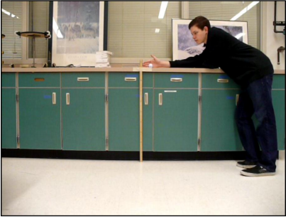
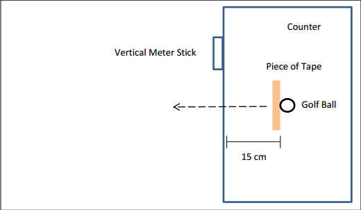
- Tape 1 meter stick to a counter so that the meter stick is in an upright, vertical position in order to measure a ball’s height when dropped.3
- Place a piece of tape on the top of the counter, 15 cm from and parallel to the edge of the counter, and mark that location for it will be from where golf balls will be pushed off of the counter.
- Place the camera on a stable surface so that the camera’s view can see the entirety of the experiment’s setup within its frame.
- Select three golf balls that have been at room temperature (20.5 ± 1 °C) and set them aside.
- Select one of the three room temperature golf balls and set it behind the starting line, 15 cm back from the edge of the counter.
- Commence the camera’s video recording by pressing the appropriate button.
- Gently push the golf ball off of the counter, towards the camera.
- Once the golf ball has bounced twice, stop the camera’s video recording by pressing the appropriate button.
- Repeat steps 17 – 20 with the same golf ball twice for a total of three trials per golf ball.
- Repeat steps 17 – 21 with each of the other two room temperature golf balls.
- Repeat steps 17 – 21 with each of the dry ice golf balls.
- Repeat steps 17 – 21 with each of the 100 ± 1 °C golf balls.
- Repeat steps 17 – 21 with each of the 73.5 ± 1 °C golf balls.
- Manipulate the temperature of the first beaker (100 ± 1 °C) in order to achieve a temperature of 61.0 ± 1 °C. This may involve sublimating a small amount of dry ice in the beaker in order to cool the water.
- Manipulate the temperature of the second beaker (73.5 ± 1 °C) in order to achieve a temperature of 17.5 ± 1 °C. This may involve sublimating a small amount of dry ice in the beaker in order to cool the water.
- Place three golf balls into each beaker when the water temperature of each stabilizes at the aforementioned values.
- Repeat steps 17 – 20 with each of the 61.0 ± 1 °C golf balls.
- Repeat steps 17 – 20 with each of the 17.5 ± 1 °C golf balls.
- Clean-up setup and put away all materials.
- Analyze each video with LoggerPro in order to determine each ball’s drop and return heights.
Illustrations and Diagrams
Data
Collected and Raw Data4
| Ball Type / Temperature (°C) | Ball | Trial | Initial Height (m) | Final Height (m) |
|---|---|---|---|---|
| Room Temp (20.5 ± 1 °C) | 1 | 1 | 1.520 | 1.309 |
| Room Temp (20.5 ± 1 °C) | 1 | 2 | 1.536 | 1.294 |
| Room Temp (20.5 ± 1 °C) | 1 | 3 | 1.545 | 1.317 |
| Room Temp (20.5 ± 1 °C) | 2 | 1 | 1.555 | 1.338 |
| Room Temp (20.5 ± 1 °C) | 2 | 2 | 1.550 | 1.328 |
| Room Temp (20.5 ± 1 °C) | 2 | 3 | 1.532 | 1.293 |
| Room Temp (20.5 ± 1 °C) | 3 | 1 | 1.577 | 1.352 |
| Room Temp (20.5 ± 1 °C) | 3 | 2 | 1.554 | 1.311 |
| Room Temp (20.5 ± 1 °C) | 3 | 3 | 1.527 | 1.299 |
| Dry Ice (-78.5 ± 1 °C) | 1 | 1 | 1.516 | 1.118 |
| Dry Ice (-78.5 ± 1 °C) | 1 | 2 | 1.512 | 1.152 |
| Dry Ice (-78.5 ± 1 °C) | 1 | 3 | 1.548 | 1.183 |
| Dry Ice (-78.5 ± 1 °C) | 3 | 1 | 1.545 | 1.194 |
| Dry Ice (-78.5 ± 1 °C) | 3 | 2 | 1.558 | 1.213 |
| Dry Ice (-78.5 ± 1 °C) | 3 | 3 | 1.545 | 1.172 |
| Boiling (100 ± 1 °C) | 1 | 1 | 1.582 | 1.184 |
| Boiling (100 ± 1 °C) | 1 | 2 | 1.553 | 1.169 |
| Boiling (100 ± 1 °C) | 1 | 3 | 1.598 | 1.240 |
| Boiling (100 ± 1 °C) | 2 | 1 | 1.600 | 1.217 |
| Boiling (100 ± 1 °C) | 2 | 2 | 1.577 | 1.197 |
| Boiling (100 ± 1 °C) | 2 | 3 | 1.544 | 1.227 |
| Boiling (100 ± 1 °C) | 3 | 1 | 1.593 | 1.198 |
| Boiling (100 ± 1 °C) | 3 | 2 | 1.591 | 1.181 |
| Boiling (100 ± 1 °C) | 3 | 3 | 1.561 | 1.160 |
| Ball Type/Temeprature (°C) | Ball | Trial | Initial Heigh (m) | Final Height (m) |
|---|---|---|---|---|
| Hot (73.5 ± 1 °C) | 1 | 1 | 1.572 | 1.355 |
| Hot (73.5 ± 1 °C) | 1 | 2 | 1.569 | 1.361 |
| Hot (73.5 ± 1 °C) | 1 | 3 | 1.565 | 1.367 |
| Hot (73.5 ± 1 °C) | 2 | 1 | 1.569 | 1.362 |
| Hot (73.5 ± 1 °C) | 2 | 2 | 1.566 | 1.362 |
| Hot (73.5 ± 1 °C) | 2 | 3 | 1.577 | 1.376 |
| Hot (73.5 ± 1 °C) | 3 | 1 | 1.580 | 1.345 |
| Hot (73.5 ± 1 °C) | 3 | 2 | 1.544 | 1.340 |
| Hot (73.5 ± 1 °C) | 3 | 3 | 1.565 | 1.362 |
| Mild (61.0 ± 1 °C) | 1 | 1 | 1.542 | 1.339 |
| Mild (61.0 ± 1 °C) | 1 | 2 | 1.562 | 1.365 |
| Mild (61.0 ± 1 °C) | 1 | 3 | 1.569 | 1.371 |
| Mild (61.0 ± 1 °C) | 2 | 1 | 1.574 | 1.371 |
| Mild (61.0 ± 1 °C) | 2 | 2 | 1.576 | 1.355 |
| Mild (61.0 ± 1 °C) | 2 | 3 | 1.520 | 1.286 |
| Mild (61.0 ± 1 °C) | 3 | 1 | 1.573 | 1.376 |
| Mild (61.0 ± 1 °C) | 3 | 2 | 1.592 | 1.361 |
| Mild (61.0 ± 1 °C) | 3 | 3 | 1.546 | 1.356 |
| Cold (17.5 ± 1 °C) | 1 | 1 | 1.572 | 1.325 |
| Cold (17.5 ± 1 °C) | 1 | 2 | 1.589 | 1.374 |
| Cold (17.5 ± 1 °C) | 1 | 3 | 1.559 | 1.339 |
| Cold (17.5 ± 1 °C) | 2 | 1 | 1.590 | 1.355 |
| Cold (17.5 ± 1 °C) | 2 | 2 | 1.583 | 1.383 |
| Cold (17.5 ± 1 °C) | 2 | 3 | 1.563 | 1.344 |
| Cold (17.5 ± 1 °C) | 3 | 1 | 1.565 | 1.333 |
| Cold (17.5 ± 1 °C) | 3 | 2 | 1.588 | 1.362 |
| Cold (17.5 ± 1 °C) | 3 | 3 | 1.586 | 1.376 |
Calculations and Processed Data
![Coef[rest]=height[d]/height[r]](img/calc1.png)
![Where Coef[rest] is the Coefficient of Restitution (constant, scalar, no units); Height[d] is t he initial drop height of the golf ball in meters, height[r] is the return height of the golf ball in meters.](img/calc2.png)
![Avrg[Coef[Rest]] = n^-1 * SIGMA(Coef[rest],n,1) Where Avrg[Coef[Rest]] is the Coefficient of Restitution (constant, scalar, no units), n is the total number of golf ball drops for a specific temperature, Coef[Rest] is the Coefficient of Restitution (constant, scalar, no units)](img/calc3.png)
| Ball Type/Temperature (°C) | Ball | Trial | Coef. of Rest. | Avrg. Coef. of Rest. |
|---|---|---|---|---|
| Room Temp (20.5 ± 1 °C) | 1 | 1 | 0.861184211 | 0.852102 |
| Room Temp (20.5 ± 1 °C) | 1 | 2 | 0.842447917 | ↑ |
| Room Temp (20.5 ± 1 °C) | 1 | 3 | 0.852427184 | ↑ |
| Room Temp (20.5 ± 1 °C) | 2 | 1 | 0.860450161 | ↑ |
| Room Temp (20.5 ± 1 °C) | 2 | 2 | 0.856774194 | ↑ |
| Room Temp (20.5 ± 1 °C) | 2 | 3 | 0.843994778 | ↑ |
| Room Temp (20.5 ± 1 °C) | 3 | 1 | 0.857324033 | ↑ |
| Room Temp (20.5 ± 1 °C) | 3 | 2 | 0.843629344 | ↑ |
| Room Temp (20.5 ± 1 °C) | 3 | 3 | 0.850687623 | ↑ |
| Dry Ice (-78.5 ± 1 °C) | 1 | 1 | 0.737467018 | 0.762256 |
| Dry Ice (-78.5 ± 1 °C) | 1 | 2 | 0.761904762 | ↑ |
| Dry Ice (-78.5 ± 1 °C) | 1 | 3 | 0.764211886 | ↑ |
| Dry Ice (-78.5 ± 1 °C) | 3 | 1 | 0.772815534 | ↑ |
| Dry Ice (-78.5 ± 1 °C) | 3 | 2 | 0.778562259 | ↑ |
| Dry Ice (-78.5 ± 1 °C) | 3 | 3 | 0.758576052 | ↑ |
| Boiling (100 ± 1 °C) | 1 | 1 | 0.748419722 | 0.758770 |
| Boiling (100 ± 1 °C) | 1 | 2 | 0.752736639 | ↑ |
| Boiling (100 ± 1 °C) | 1 | 3 | 0.775969962 | ↑ |
| Boiling (100 ± 1 °C) | 2 | 1 | 0.760625000 | ↑ |
| Boiling (100 ± 1 °C) | 2 | 2 | 0.759036145 | ↑ |
| Boiling (100 ± 1 °C) | 2 | 3 | 0.794689119 | ↑ |
| Boiling (100 ± 1 °C) | 3 | 1 | 0.752040176 | ↑ |
| Boiling (100 ± 1 °C) | 3 | 2 | 0.742300440 | ↑ |
| Boiling (100 ± 1 °C) | 3 | 3 | 0.743113389 | ↑ |
| Hot (73.5 ± 1 °C) | 1 | 1 | 0.861959288 | 0.866961 |
| Hot (73.5 ± 1 °C) | 1 | 2 | 0.867431485 | ↑ |
| Hot (73.5 ± 1 °C) | 1 | 3 | 0.873482428 | ↑ |
| Hot (73.5 ± 1 °C) | 2 | 1 | 0.868068834 | ↑ |
| Hot (73.5 ± 1 °C) | 2 | 2 | 0.869731801 | ↑ |
| Hot (73.5 ± 1 °C) | 2 | 3 | 0.872542803 | ↑ |
| Hot (73.5 ± 1 °C) | 3 | 1 | 0.851265823 | ↑ |
| Hot (73.5 ± 1 °C) | 3 | 2 | 0.867875648 | ↑ |
| Hot (73.5 ± 1 °C) | 3 | 3 | 0.870287540 | ↑ |
| Mild (61.0 ± 1 °C) | 1 | 1 | 0.868352789 | 0.866628 |
| Mild (61.0 ± 1 °C) | 1 | 2 | 0.873879641 | ↑ |
| Mild (61.0 ± 1 °C) | 1 | 3 | 0.873804971 | ↑ |
| Mild (61.0 ± 1 °C) | 2 | 1 | 0.871029225 | ↑ |
| Mild (61.0 ± 1 °C) | 2 | 2 | 0.859771574 | ↑ |
| Mild (61.0 ± 1 °C) | 2 | 3 | 0.846052632 | ↑ |
| Mild (61.0 ± 1 °C) | 3 | 1 | 0.874761602 | ↑ |
| Mild (61.0 ± 1 °C) | 3 | 2 | 0.854899497 | ↑ |
| Mild (61.0 ± 1 °C) | 3 | 3 | 0.877102199 | ↑ |
| Cold (17.5 ± 1 °C) | 1 | 1 | 0.842875318 | 0.858803 |
| Cold (17.5 ± 1 °C) | 1 | 2 | 0.864694777 | ↑ |
| Cold (17.5 ± 1 °C) | 1 | 3 | 0.858883900 | ↑ |
| Cold (17.5 ± 1 °C) | 2 | 1 | 0.852201258 | ↑ |
| Cold (17.5 ± 1 °C) | 2 | 2 | 0.873657612 | ↑ |
| Cold (17.5 ± 1 °C) | 2 | 3 | 0.859884837 | ↑ |
| Cold (17.5 ± 1 °C) | 3 | 1 | 0.851757188 | ↑ |
| Cold (17.5 ± 1 °C) | 3 | 2 | 0.857682620 | ↑ |
| Cold (17.5 ± 1 °C) | 3 | 3 | 0.867591425 | ↑ |
| Ball Type/Temperature (°C) | Avrg. Coef. of Rest. |
|---|---|
| Dry Ice (-78.5 ± 1 °C) | 0.762256 |
| Cold (17.5 °C) | 0.858803 |
| Room Temp (20.5 ± 1 °C) | 0.852102 |
| Mild (61.0 °C) | 0.866628 |
| Hot (73.5 °C) | 0.866961 |
| Boiling (100 ± 1 °C) | 0.758770 |


The optimal temperature for the highest coefficient of restitution, using the second order trendline, can be found be taking the derivative of the second order trendline function, setting it equal to 0, and solving for x.
ƒ(x) = -0.00001x² + 0.0004x + .8674
ƒ'(x) = -0.00002x + 0.0004
0 = -0.00002x + 0.0004
0.00002x = 0.0004
x = 20.0
Therefore, the optimal temperature for the highest coefficient of restitution, using the second order trendling, is 20.0 °C.
The optimal temperature for the highest coefficient of restitution, using the third order trendline, can be found be taking the derivative of the third order trendline function, setting it equal to 0, and solving for x.
ƒ(x) = -0.0000002x³ - 0.000003x² + 0.0019x + 0.8218
ƒ'(x) = -0.0000006x² - 0.000006x + 0.0019
0 = -0.0000006x² - 0.000006x + 0.0019
x = 51.46948, -61.4948
Therefore, the optimal temperature for the highest coefficient of restitution, using the second order trendline, is 51.4948°C. Note that the solution -61.4948 is discarded, because the graph supports the conclusion that this temperature produces the lowest coefficient of restitution possible.
Conclusion
Aspect 1: Overall Conclusion
This investigation’s hypothesis was ultimately supported in that the temperature vs. coefficient of restitution graph and data points resembled a bell curve which peaked between 20 – 60 °C. Strictly according to the graph, the 73.5 ± 1 °C produced the highest coefficient of restitution. However, the difference between the coefficients of restitution produced by the 73.5 ± 1 °C temperature and the room temperature (20.5 ± 1 °C) was approximately 0.014859. Converting that value to meters by multiplying by the initial drop height, the difference between the heights produced by the 73.5 ± 1 °C temperature and the room temperature (20.5 ± 1 °C) was approximately 2.22885 cm. Therefore, this investigation concludes that temperatures within the reasonable and approximate range of 0 – 75 °C, produce extremely similar coefficients of restitution.
Additionally, according to the second order trendline, the optimal temperature for the highest coefficient of restitution was 20 °C or 68 °F. According to the third order trendline, the optimal temperature for the highest coefficient of restitution was 51.4948 °C. Thus, both of these trendlines support the hypothesis that “reasonable temperatures” (Thomas) produce the highest coefficients of restitution when compared to coefficients of restitution produced by extreme thermal values. However, because the data points do not clearly distinguish the best trendline (second order vs. third order), this investigation ventures to logically conclude that more data points would be extremely helpful in determining the appropriate graph to resemble the data points. Nevertheless, in order to determine the overall optimum temperature for the highest coefficient of restitution, this investigation averaged the optimum values provided by the second order and third order trendlines. This overall optimum temperature estimate was found to be ((20 + 51.4948) / 2) 35.7474 °C, or 96.3453 °F. Therefore, while there are noteworthy limitations to this experiment, this investigation concludes that its hypothesis was supported by the shape of the graph, the results of the data, and the approximations of the trendlines.
Aspect 2: Evaluating Procedures
There were many procedural flaws and areas for improvement in this investigation. The most prominent procedural weakness was that the experiment relied upon the assumption that the golf balls were the same temperature as that of medium in which they were placed. For example, this inquiry assumed that the temperature of the dry ice golf balls was -78.5 ± 1 °C. However, this temperature recording was that of the dry ice itself. Therefore, while the phenomenon of thermal contact and the field of thermodynamics support the assumption that the golf balls were relatively close to the temperature of their medium, this investigation must nevertheless recognize this imperfection in the procedure.
The second potential weakness was that each golf ball spent a different amount of time in its respective medium. For example, this investigation’s procedure mandated that all golf balls be placed in thermal contact with their medium, once the medium’s temperature had stabilized at the appropriate value, for 10 minutes. After 10 minutes, the procedure instructed one golf ball to be removed from the medium in order to conduct 3 trials with the golf ball. Therefore, the other two golf balls in the medium were in thermal contact with their medium for a longer duration of time than the first. It follows that the third golf ball was in thermal contact with its medium for the longest period of time, while the first golf ball was in thermal contact with the same medium for the shortest period of time. According to Newton’s Law of Cooling, heat transfer occurs extremely quickly after immediate thermal contact and gradually slows after thermal contact has been experienced for some time. Thus, while this investigation discounts the possibility of this procedural error altering the entirety of the results and conclusion, it must be noted that placing an experiment’s objects in a respective medium for varying amounts of time is a potential procedural flaw.
The most practical weakness in this investigation’s procedure is that three trials were conducted with each golf ball. Accordingly, the golf ball contained more heat, and therefore energy, during the first trial than during the third trial. This is a significant possible error due to Newton’s Law of Cooling. Apart from the aforementioned aspects of Newton’s Law of Cooling, this law also states that the rate of change of heat transfer is dependent upon the difference between the environment and the object. For example, if a relatively hot object (15 – 20 °C) was placed in a relatively cold environment (0 – 5 °C), then the object would lose heat at a relatively slow rate, because the difference between the object and the environment is relatively small. Therefore, when the extremely cold dry ice golf balls (-78.5 ± 1 °C), in this experiment, were placed in a room temperature environment (20.5 ± 1 °C), the balls would gain heat relatively quickly. Additionally, when the extremely hot golf balls (100.5 ± 1 °C), were placed in a room temperature environment (20.5 ± 1 °C), the balls would lose heat relatively quickly. Thus, the danger that this procedure incurred was that three trials with each golf ball provided each golf ball with the opportunity to have an extremely different heat content during the third trial than during the first. Because the three trials of each golf ball took less than 2 minutes to complete, the thermal difference between the first and third trial is predicted to be relatively low. Nevertheless, this investigation must recognize this potential procedural flaw.
Aspect 3: Improving the Investigation
There are several measures that could be taken in order to improve the aspects of this investigation. Firstly, placing 9 golf balls in each thermal medium would provide the same amount of data for each medium when compared to placing 3 golf balls in each medium and performing 3 trials with each golf ball. The advantage to using 9 golf balls in each medium, instead of 3, is that only one trial would be performed on each golf ball. This would eliminate the potential thermal difference between a golf ball’s first and third trials as only one trial per golf ball would occur. This, in turn, would provide more accurate and reliable results.
Secondly, this investigation would be improved if the experiment was conducted in the conditions of Standard Temperature and Pressure8. For practicality, this investigation was conducted in an environment with a temperature of 20.5 ± 1 °C (68.9 ± 1.8 °F) and a pressure of 1.00 atm (in absolute pressure). Because these conditions significantly differ from the conditions of Standard Temperature and Pressure, this investigation would produce more reliable and standardized results if the experiment was conducted in the conditions of Standard Temperature and Pressure.
Furthermore, another potential improvement to this investigation is for the golf balls to be placed in their respective mediums for a longer duration of time than 10 minutes. While this would ensure that the golf balls are relatively close to the temperature of the medium, Newton’s Law of Cooling assured this investigation that 10 minutes would suffice for the temperature differences that this investigation used. Note that Newton’s Law of Cooling, it its differential form, is  .
.
Finally, the largest improvement that could be made to this investigation is to use an insulated thermal contact probe in order to quickly measure the temperature of the golf ball. This would reduce the discrepancy between measuring the medium of the golf ball and assuming that the golf balls share the temperature of their medium. Ultimately, this investigation concludes that these potential procedural flaws did not severely affect the results of this experiment. However, the improvement of this investigation and its procedure could yield more effective results.